¶ 1. Summary
The T6 Planning manual provides a comprehensive overview of the use of formulas and functions in the software, highlighting the versatility from simple calculations to advanced operations. It explores the automatic execution of formulas in response to data changes, including the ability for manual execution through a wizard. The performance chapter provides practical tips for optimizing the use of formulas, identifying bottlenecks and problems in cycles. Additionally, the manual covers the available functions and parameter types, seeking to provide users with a detailed understanding of the properties and characteristics of formulas for efficient use in the context of T6 Planning.
¶ 2. Formulas and Functions
The formulas module allows you to write all business rules according to the mapping created from the Excel model. Whenever possible or necessary, support accounts will be created to demonstrate the calculation memory of the accounts, however this is not a rule and one can opt for the direct calculation of an account when this form is more mathematically optimized or when an internal function is already available.
¶ 2.1 Overview
The T6 Planning formulas are a powerful tool for performing calculations on model data.
T6 Planning allows from the creation of simple formulas with basic operations to complex formulas with conditionals or advanced calculations. Additionally, it offers the user a wide range of ready-made functions to further assist in the elaboration and creation of complex calculations. This manual describes in detail the properties and characteristics of the formulas available in the T6 Planning solution, aiming to provide a greater understanding of the use of advanced settings.
¶ 3. Formulas
¶ 3.1. Overview
In this topic we will explain a little more about what the structure and creation of T6 formulas are, their characteristics and functionalities.
Formulas are very important tools for performing calculations on data and through them T6 makes it possible to perform advanced manipulations on data stored in Fact tables.
¶ 3.2. Prerequisites
In order to create, view and execute formulas within T6, we will need to have the following features enabled:
User Features
- Manager:
- Manage application structure/model;
- Analyst:
- View formula;
Global group feature
¶ 3.2.1. Formula Structure
The basic structure of a formula consists of four configuration steps, which are displayed as tabs in the formula panel, namely Formula, Scope, Description and Data.
¶ 3.2.2. Formula
It is the first step in the formula creation process. Mandatory; Within formula, we will have Application, Type, Formula Group, Position, Formula Name and Expression;
-
Application: Field that informs which application the formula will be created in. After creation it will no longer be possible to edit this information;
-
Type: Mandatory field where the type of formula is selected:
- Special: Formulas that calculate in the entire scope in which they were configured or when changes impact members present in it;- In-Memory: Formulas that are not persisted in the database. They are calculated only in the scope visible to the user in the form or report. They are useful for point calculations;
-
Formula Group: Optional field where the formula group will be selected (functionality to group formulas within T6, used to organize formulas by context, category or purpose);
-
Position: Non-editable field; Indicates the positioning of the formula in relation to others; The positioning refers to the order in which formulas will be executed, it is automatically generated by T6 during cube publication;
T6 takes into account new formulas created or possible changes that have occurred in existing formulas. It is possible to manually sort formulas in the Formula List, however, when publishing the Cube, T6 will reposition them according to the best execution order.
Example:
| Position | Formula |
|---|---|
| 1 | [A] = [B] + [C] |
| 2 | [B] = [D] + [E] |
The formula at position 1 has a member [B] that is calculated by another formula. However, by ordering, the formula that calculates [B] is in the second position. When publishing the Cube, T6 will automatically reposition the formula [B] = [D] + [E] before the formula [A] = [B] + [C], because only after calculating [B] will it be possible to calculate the value of [A].
-
Formula Name: Mandatory field, must be filled with the formula name.
- Tip: Always try to use a name that refers to the objective of the formula, for example, "Calculation of labor taxes"; -
Expression: Field where the formula detail is performed, represents the expression that the formula will execute. It resembles a mathematical expression, contains an operand being equated to a sequence of operands and operators interspersed, always starting and ending with an operand.
Example:
[C1] = [C2] + [C3]
[C1]: Operand that will receive the result of the expression. This operand is also known as the resultant operand;
[C2]: Operand that will be used in the calculation of the expression;
+ : Operator to be used in the calculation of the expression;
[C3]: Operand that will be used in the calculation of the expression.
In this example, the value of [C1] will be equal to the value of [C2] plus the value of [C3].
In an expression, operands can be: Member, Number, Function and Block;
The resultant operand must necessarily be a member, which may or may not have scope.
Among the operators we have: Sum (+), Subtraction (-), Multiplication (*), Division (/) and Power (^);
In the expression field, we can use autocomplete by typing at least 3 characters (after 1 second the suggestions will be displayed), or by clicking CTRL + SPACE which will display suggestions for insertion.
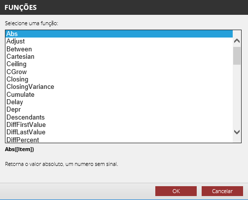
We have a button that displays the available Functions for selection:
.
Functions are helpers for creating formulas, allowing more elaborate calculations, in addition to providing access to various model information.
For additional information regarding functions in T6, access: Formulas and Functions
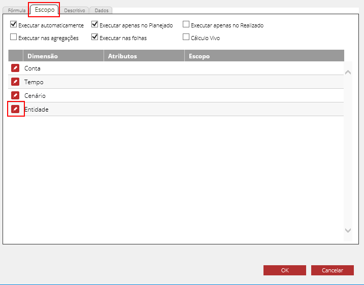
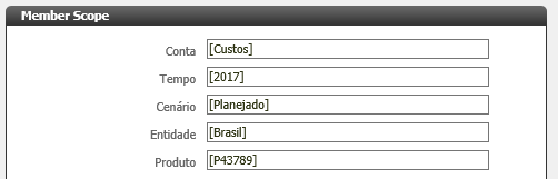
¶ 3.2.3. Scope
Allows filtering the execution context of a formula. With this, the execution of the formula will be performed according to the inserted filters.
Using the scope it is possible to filter in which dimension members the formula will be executed. If no filter is inserted in the dimension, the formula will be executed in all members.
The execution filters in the scope tab are displayed as checkboxes, in the filters we will have:
- Execute Automatically: Allows executing the formula automatically when saving data in a form.
Formulas with this property active are called Online Formulas; Formulas in which the property is disabled are called Offline Formulas.
Whenever a formula premise has its value changed, directly or indirectly, the formula will be executed, changing its values, thereby making the formula expression true again.
-
Execute Only in Planned: This option is available only in Planning applications and allows executing the formula only in the planned scenario. When this property is active, the formula calculation will be performed only in the periods configured as planned.
-
Execute Only in Actual: This option is available only in Planning applications and allows executing the formula only in the actual scenario. When this property is active, the formula calculation will be performed only in the periods configured as actual.
If you wish to run the formula in both scenarios, Planned and Actual, uncheck both checkboxes.
-
Allow Persist Zero: When we select the checkbox, the formula can save the zero value in the fact; Normally, in T6 the zero value is not saved in the fact, but in some specific cases this is necessary.
-
Execute in Aggregations: This option is available only for In-Memory type formulas. When this property is active, the formula calculation will be performed at aggregated levels.
-
Execute in Leaves: This option is available only for In-Memory type formulas. When this property is active, the formula calculation will be performed at leaf levels.
-
Live Calculation: When this property is active, the formula calculation will be performed whenever one of the premises is changed by the user, without the need to save the data.
¶ 3.2.4. Description
Allows describing the function of the formula or its objectives, in order to provide a detailed description of the formula.
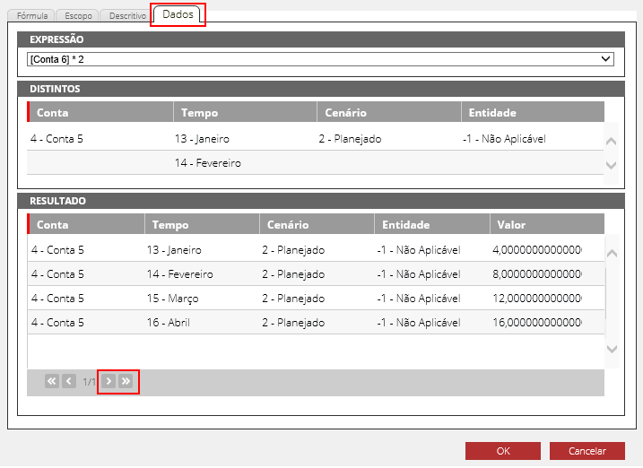
¶ 3.2.5. Data
Allows viewing information regarding the formula's execution scope, making it possible to analyze each expression generated by the formula and viewing data from these expressions. In the data tab, we have Expression, Distinct and Result;
-
Expression: In expression, we can see the formula execution scope, displaying each of the premises separately;
-
Distinct: In distinct, we can view the unique combination of members changed by the expression, in distinct we will have Account, Time, Scenario and Entity, so we can view where the data is being changed by that expression;
-
Result: In result, we can preview the data we have in the model based on the selected expression;
¶ 3.3. Formula Creation
To create a new formula, follow these steps:
- In the T6 main menu, double-click on the Explorer option;
- Select the location where the new formula will be created;
- After selecting the location, in the ribbon click New Item, click Modeling and select the Formula option;
- A new object of type Formula will be displayed in the list;
- Select the created object and click
 ;
; - A panel will open on the side with four tabs (Formula, Scope, Description and Data);
- In the Formula tab, we will have the following fields to fill in:
- Application: Indicates the application in which the formula will be created;
- Type: Indicates the type of formula (Special or In-Memory);
- Formula Group: Optional field, where we can select a group for the formula;
- Position: Indicates the positioning of the formula in relation to others. The positioning refers to the execution order of the formulas (non-editable, will be changed according to the execution order defined in the formula list);
- Formula Name: Field where we can change the formula name, by default, it brings the name defined when creating the object in Explorer;
- Expression: Mandatory field, where we must inform the formula detail;
- If necessary, to assist in filling in the formula text, we can use the fill wizard. To do this, we will press CTRL + SPACE, and view the possible alternatives according to the current context of the expression;
- Search Function: Allows us to choose a function to be used in the formula. By choosing this option, we will be directed to the list of available functions, where we will select the desired function and be directed to the function editing screen where we will add the function parameters (also has a fill wizard, with the options Search dimension and Search account member);
- Search Dimension: Displays a list with the existing dimensions in the Application and allows us to select a dimension;
- Search account member: Allows us to select a member of the account dimension, whether it is a parent member or a child member. The members are displayed in the form of a hierarchical tree;
Every new formula receives an automatic temporary positioning. After publishing the cube, T6 automatically adjusts the positioning of all formulas.
With the expression configured we can proceed to the scope, there is no impediment to navigate between tabs, however, to configure the scope we need to have the expression configured.
- In the Scope tab we will check the checkboxes corresponding to the type of filter we want to enable in the formula execution, we have the following checkboxes:
- Execute automatically: Allows executing the formula automatically when saving data in a form;
- Execute in aggregations: This option is available only for In-Memory type formulas. When this property is active, the formula calculation will be performed at aggregated levels;
- Execute only in planned: This option is available only in Planning applications and allows executing the formula only in the planned scenario;
- Execute in leaves: This option is available only for In-Memory type formulas. When this property is active, the formula calculation will be performed at leaf levels;
- Execute only in actual: This option is available only in Planning applications and allows executing the formula only in the actual scenario;
- Live calculation: When this property is active, the formula calculation will be performed whenever one of the premises is changed by the user, without the need to save the data;
- Allow persist zero;
- Still in the Scope tab, we will click on the dimension row we want to select and then click on
 to select the members and attributes that will compose the formula scope;
- The list with the members of the selected dimension will be displayed, where members and attributes can be selected for filtering.
- In the Description tab we will describe the purpose of the formula or its objectives;
- In the Data tab we will view the information regarding the formula's execution scope (this screen is widely used to identify possible errors or problems in formula calculations);
- Still in the Data tab, we will have the fields Expression, Distinct and Result;
- Expression: The Expression field displays a list with all the expressions of the operands and blocks of operands of the formula.
- For example: in a formula
A = B + C,B,CandB + Cwill be displayed in the list;- Distinct: Displays a list with the distinct values of the tuples where data exists for the selected expression;
- Result: Displays a list with the values found in various tuples for the selected expression.
After creating a formula, it is necessary to publish the cube so that it can be used!
¶ 3.4 Accessing the Application Formulas
The list of existing formulas in the application can be accessed from the T6 Planning main screen, through Menu -> Modeling -> Formulas.

The system will display the Formulas screen, which contains the listing of all the application's formulas.

¶ 3.5 Configuration and Use of Features
Formula configuration is done from the Formulas screen.
This screen contains several features and, among other functions, will allow you to sort, add, edit, remove and execute formulas, as well as view cycles or intersections in the formulas.
For a better understanding, observe the numbered and highlighted features in the image below, and then follow the details and use of each feature.
-
Formula List: This is a grid that displays the listing of formulas existing in the model and contains the following columns:
- Pos: Indicates the positioning of the formula in relation to others. The positioning refers to the order in which the formulas will be executed.
- Type: Indicates the type of the formula (Special or In-Memory).
- Group: Formula group.
- Name: Name that identifies the formula.
List configuration and use of features:
- To configure a particular formula, simply double-click on it in the formula list. The Formula Creation and Editing screen will be displayed. For more details, see the Create and Edit Formulas topic in this Manual.
- To use the features located at the bottom of the screen, where the Action Menu and Action Buttons are located, it is necessary to first select a particular formula in the list by clicking once on it. Then click on the desired feature.
- To use the features of the Tools Menu, located at the top of the screen, there is no need for a prior selection in the formula list, since the use of such options reflects on all formulas in the list.
-
Type: This is a combobox that allows filtering the formulas based on the selected type, displaying only the formulas related to the selected group.
-
Formula Group: This is a combobox that allows filtering the formula list based on the selected Group, displaying only the formulas related to the selected group.
-
Application: This is a combobox that allows filtering the formulas based on the selected application, displaying only the formulas related to the selected application.
-
Execute formulas automatically: This is a checkbox, which should be unchecked when you want to temporarily disable the automatic execution of formulas. The use of this feature reflects on the entire formula list.
-
Action Buttons: These are the buttons located in the lower right corner of the screen.
Use of buttons:
- The use of such buttons implies first selecting an item in the formula list by clicking once on a particular formula and then clicking on the desired button.
Button options:
- Add: Allows creating and adding a new formula to the existing list. When you click the button, the Formula Creation and Editing screen will be displayed. For more details see the Create and Edit Formulas topic in this manual.
- Edit: Allows editing an existing formula in the list. When you click the button, the Formula Creation and Editing screen will be displayed. For more details, see the Create and Edit Formulas topic in this manual.
- Remove: Allows removing a previously selected formula from the list.
- History: Displays all executions of a previously selected formula in the list. For more details, see the Model History topic in the Formula Execution chapter of this manual.
-
Actions Menu: This is the options menu located in the lower right corner of the screen.
Actions menu options:
- Move Up: Allows moving a previously selected formula in the list to a position above the current one.
- Move Down: Allows moving a previously selected formula in the list to a position below the current one.
-
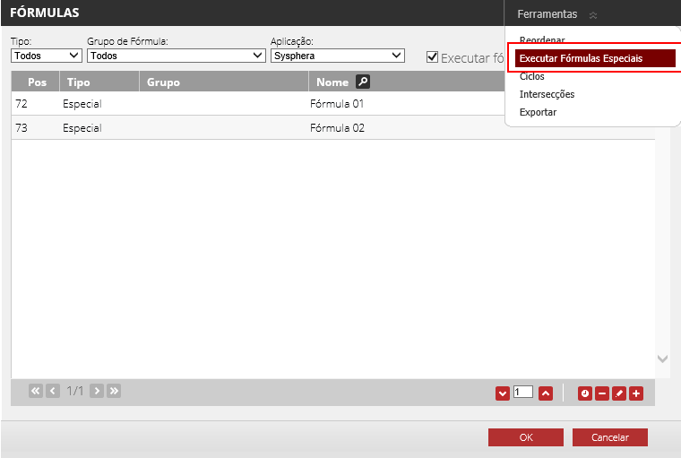
Tools Menu: This is the options menu located in the upper right corner of the screen. The tools menu contains features that, when used, automatically affect all content in the formula list. Therefore, there is no need to make a prior selection of a particular formula in the list.
Tools menu options:
- Reorder: Allows automatically reordering all formulas, taking into account their precedence and always reporting when any circular reference occurs.
- Execute Special Formulas: Allows executing one or more formulas. By clicking on this option you will start the Formula Execution Wizard. For more details, see the Special Formula Execution topic in the Execution chapter of this manual.
- Cycles: Displays formulas that have cycles. For more details, see the Cycles topic in the Performance chapter of this manual.
- Intersections: Displays formulas that have Intersections. For more details, see the Intersections topic in the Performance chapter of this manual.
¶ 3.6 Create and Edit Formulas
Use this feature to create a new formula or change the properties of an existing formula.
- To Add Formula: On the Sort Formulas screen, use the Add button, located in the lower right corner of the screen.
- To Edit Formula: On the Sort Formulas screen, select the formula you want to edit by clicking on it in the formula list. Then click the Edit button, located in the lower right corner of the screen.
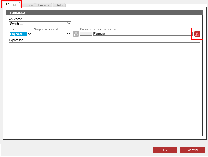
The Add and Edit buttons are highlighted in the image above. When you click the Add or Edit buttons, the Formula screen will be displayed. This screen contains the 4 formula configuration steps, as highlighted in the image below.
To start the configuration, both for Adding and Editing a formula, use the following steps:
On the Formula screen – FORMULA Tab:
-
Application: Indicates which application the formula was created in.
-
Type: Indicates the type of the formula.
-
Formula Group: Optional field in which you can select a group for the formula.
-
Position: Indicates the positioning of the formula in relation to others. The positioning refers to the order in which the formulas will be executed.
-
Formula Name: Mandatory field where you must enter the name of the formula.
-
Functions: Its use is linked to the Expression field. When you click on this field, the Function List screen will be displayed. You can select a function, considering your need based on its description. For more details on the existing functions, see the Functions Chapter in this manual.
-
Expression: Mandatory field, where the formula detail must be provided. Note some points that will facilitate the detailing:
- If you want to choose a function to fill in the formula expression, simply click the Functions button, located in the upper right corner of the screen. Check the list of available functions in the Functions chapter.
- If you need help filling in the formula text, you can use the fill wizard. For this, press Ctrl + space, and view the possible alternatives according to the current context of the expression. Note that:
- Search Function: Allows you to choose a function to use in the formula. By choosing this option, you will be directed to a list of available functions. After choosing the desired function, you will be directed to the "Function Editing" screen which allows editing the parameters of a function.
- Member Scope Editing: Allows editing the member scope.
- Search Member or Dimension: Allows searching for a member or dimension.
In the image below, the red highlights point to the mandatory fields. The blue highlight shows the fill wizard for the Expression field.
Note that every new formula receives an automatic temporary positioning. After publishing the Cube, T6 Planning will adjust the positioning of all formulas.
To finish, click OK. The formula list will be updated.
On the Formula screen – SCOPE Tab:
- Check the checkbox corresponding to the type of filter with which you want to execute the formula. For more details on filters, see the Scope topic in the Formulas chapter of this manual.
- Click on the dimension row to select it. Then, click the Edit button and select the members that will compose the scope. Thus, the list will present the Dimension Name, the Scope (or Members) and the Selected Attributes.
On the Formula screen – DESCRIPTION Tab:
- In the Description field, describe the purpose of the formula or its objectives.
On the Formula screen – DATA Tab:
- On this screen you only view information regarding the formula's Execution Scope. It is possible to analyze each expression generated by the formula and view data from these expressions. This screen is widely used to identify possible errors or problems in formula calculations. For more details, see the Identifying Problems in Cycles topic in the Performance chapter of this manual.
- The Expression field displays a list with all the expressions of the operands and blocks of operands of the formula. For example: in a formula A = B + C, A, B and A + B will be displayed in the list.
- The Distinct field displays a list with the distinct values of the tuples where data exists for the selected expression.
- The Result field displays a list with the values found in various tuples for the selected expression.
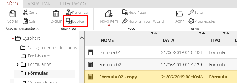
¶ 3.6.1 Duplicating a Formula
Aiming to facilitate the copying of formulas without changing the original structure, T6 Planning provides a button that allows a new formula to be created, identical to the current one. The Duplicate button allows replicating a formula and optimizing formula creation time.
- In the formula list, click on the formula you want to duplicate, and in the options bar click the Duplicate button.
- The duplicated formula will be displayed in the formula list. Rename it.
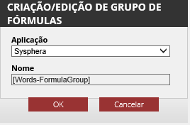
¶ 3.7 Create and Edit Formula Groups
Use this feature to create formula groups and better organize Formulas by context, categories or purpose.
To add a Formula Group:
-
In the T6 Planning menu, access Explorer -> Navigator.
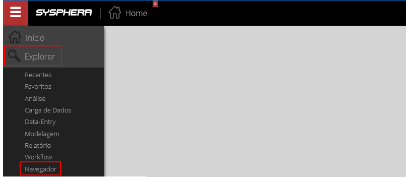
-
On the left side of the screen, you will find the system folders listing.
-
Select the folder in which you want to save the Formula Group.
-
In the options bar, click New Item, expand the Modeling item by clicking on it, and then click Formula Group.
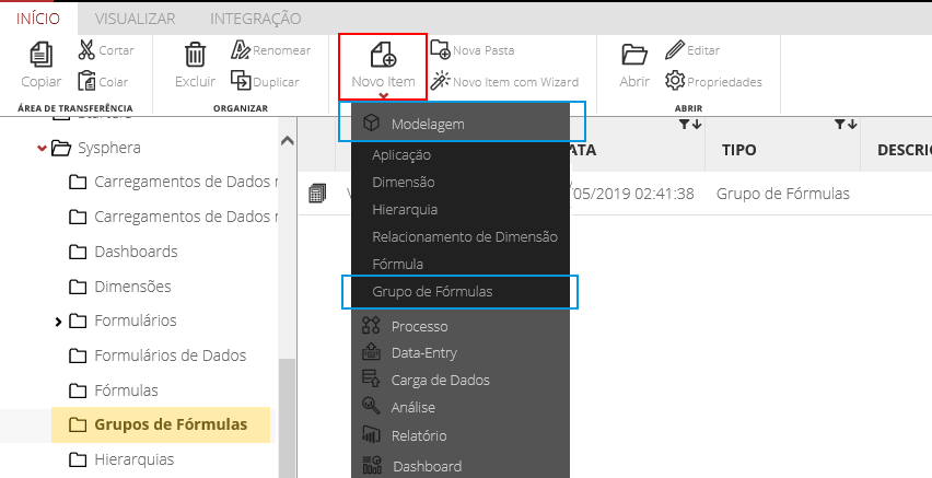
-
The new Formula Group will appear in the center of the screen, in the formula group list.
-
Name the group.
To Edit a Formula Group:
-
In the formula group list, select the Formula Group you want to edit by clicking on it.
-
Then, in the options bar, click the Edit button.
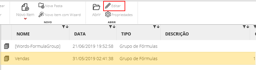
-
A pop-up window will be displayed. The application field is already set, you must then enter the name of the group being created, with the Name field being mandatory. Then click Ok.
¶ 4. Formula Execution
¶ 4.1 Overview
Whenever a data change or insertion is performed, T6 Planning identifies the formulas involved in the calculation of this data and executes them. If there is a dependency between any of these formulas, it will also be executed.
T6 Planning uses this identification system to prevent all other existing formulas from being recalculated without any changes having occurred in the data.
This chapter will show how cycles, dependencies, parameters and formula execution work in T6 Planning.
¶ 4.2 Dependencies, Cycles and Recursions
When the application has several formulas that interact with each other, or when there is a dependency between them, this set of formulas is called a cycle.
When publishing the cube, T6 Planning sorts the formulas according to dependencies. If the formula is in a cycle, the formula will remain in the same position relative to the formulas that are in the cycle. That is, the formulas must be sorted within a cycle manually.
Formula cycles can be viewed at: -> Sort Formulas window -> Tools -> Cycles. This view is used to verify when a cycle is accidentally created and in case it is necessary to delete a formula, knowing where that will have an impact.
Example:
In an application we have the members: A, B and C, and we will create two formulas:
Formula 1:
[C] = [A] + [B]
Formula 2:
A = Lag([C], -1)
(Click on the following link if you have questions about the Lag Function.)
-
After publishing them we will return to the formulas screen.
-
In tools, within the formulas screen, we will have the Cycles option. When we click on it, the existing cycles between the formulas will be displayed.
In the cycle display, we will have the formulas we created earlier, and next to their name, a number in parentheses, which will define the dependency link between the formulas.
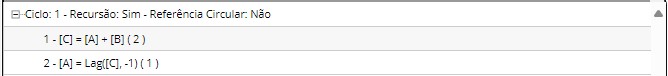
It is also displayed, next to the cycle name, whether we have Recursion and/or Circular Reference.
We have an application parameter called Maximum Iteration in Formulas that has a default value of 1. Changing this value can generate a large performance loss in your application.
¶ 4.2.1 Dependencies Between Formulas
The dependency between formulas can be characterized as direct or indirect, according to the paths between the formulas.
- Direct: When a formula depends on the form premises after the data is saved, to be executed. For example, when entering data in a form that calculates the total of monthly expenses.
- Indirect: When the calculation of one result depends on the calculation of another, to be executed. For example, a form that calculates the total of annual expenses, based on the sum of monthly expenses.
¶ 4.2.2 Formula Cycles
A cycle is a group of formulas where their execution can occur with recursion and/or circular reference.
¶ 4.2.3 Formula Recursion
Recursion is a path of mutual dependency in a cycle where variations occur in the model dimensions, and where all the formulas in the cycle are executed for each leaf member of the dimension, changing only the result in that context.
In the execution of a cycle with recursion, for each leaf member of the dimension, all formulas in the cycle are executed. We can cite as an example the Time dimension, which may present a reference to a previous period, executing all formulas in the cycle month by month, and containing calculations where the opening balance of the current month is the result of the closing balance of the previous month. The closing balance of the current month, in turn, will be the opening balance plus any movement.
When it is a recursion, we have at least one path where we need to switch a dimension member horizontally — that is, when we have a Lag, the connection point between the formulas is a Lag, meaning we are moving sideways in a context, iterating over members at the same level in a dimension. (If no dimension is defined, Lag automatically selects the Time dimension.)
- When running, the recursion substitutes the formula text and runs from the first valid month through the last valid month, in the order of the cycle's formulas.
EXAMPLE:
([C],[2024].[Janeiro]) = ([A],[2024].[Janeiro]) + ([B],[2024].[Janeiro])
- The calculation will be performed in the specific context of the month, always when we do not have the time dimension, or a function, involved.
([A],[2024].[Janeiro]) = ([C],[2023].[Dezembro])
Recursion makes formula execution slower as the number of periods to be calculated increases — the more periods, the slower.
¶ 4.2.4 Formulas with Circular Reference
When a formula depends on another without any variation in the dimension, a circular reference occurs. When executing a cycle with a circular reference, all formulas in the cycle are executed N times, where N is defined in the application parameters table via the MaximumFormulasIteration parameter, which defaults to 1.
This parameter specifies the maximum number of iterations used to resolve formulas with circular references. While the resulting values continue to change during execution, T6 Planning will keep iterating; therefore, it is ideal that this parameter remains at its default value of 1, since in most cases a single iteration is sufficient for T6 Planning to resolve the circular reference.
There are some operations where we want to perform multiple calculations in the same month; however, there is no horizontal interaction in the dimension, but the calculation will change according to the number of iterations used.
For example: In the case of the Time dimension, when all formula calculations occur within the same month. In this case, the system executes the formulas for all months multiple times, as the iterations progress.
¶ 4.2.5 Intersection
An intersection occurs when two or more formulas calculate the same cell in a form.
Through the formula wizard, under tools, you can select the intersection option, which will list the formulas that are calculating the same point in the cube.
WE NEVER WANT TO HAVE INTERSECTIONS IN THE MODEL!
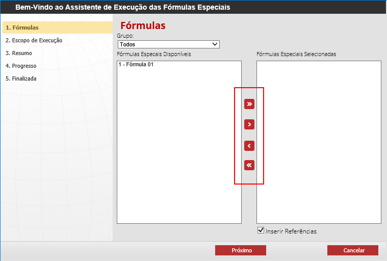
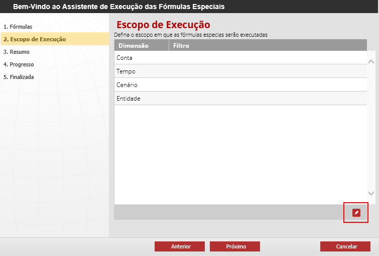
¶ 4.3 Formula Execution Wizard
This feature allows you to manually execute one or more formulas in the model. To use it, follow the steps below.
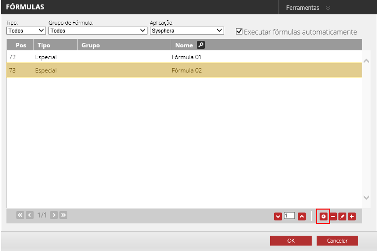
On the Formulas screen:
- In the upper-right corner of the screen, in the Tools menu, click the Execute Special Formulas option.
On the Special Formula Execution Wizard screen – FORMULAS step:
- If you want to display only the formulas of a specific group, select it from the Group dropdown.
- The Available Special Formulas field displays the list of formulas available for execution.
- The Selected Special Formulas field displays the list of formulas selected for execution.
- To add a formula, click on it and use the central navigation buttons, which allow you to add or remove a selected formula, or all formulas at once.
- Check the Insert References checkbox if you want to insert, at runtime, formulas that reference the selected formulas. This way, if the user forgets or does not add such formulas to the execution list, T6 Planning will insert them automatically to ensure consistency in the calculated values.
- To proceed, click Next.
On the Special Formula Execution Wizard screen – EXECUTION SCOPE step:
- If you want to restrict the execution scope of the formula, select it from the list of each respective model dimension.
- To configure the scope of a specific dimension, select it and then click the Edit button in the lower-right corner of the grid.
- To proceed, click Next.
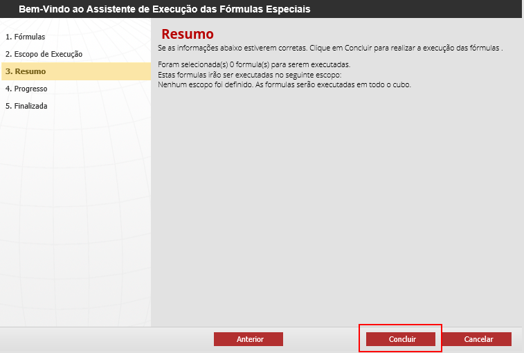
On the Special Formula Execution Wizard screen – SUMMARY step:
- Confirm the selected formulas and their execution scope.
- To proceed, click Finish.
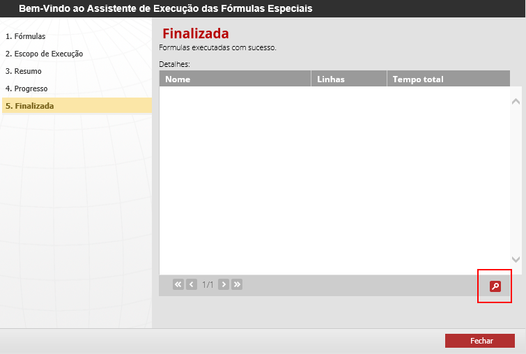
On the Special Formula Execution Wizard screen – COMPLETED step:
- This final step will display a message confirming that the formulas were executed successfully.
- To view details about the execution of a formula, select it in the list and click the View Details button in the lower-right corner of the screen.
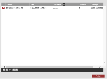
¶ 4.4 Model History
This feature displays the list of executions for a given formula, allowing analyses to identify which formulas are consuming the most time.
On the Formulas screen:
- To view the executions of a formula, select it in the list and then click the History button located in the lower-right corner of the screen.
- A popup will open showing all executions of the formula.
On the Formula Execution screen, a list displays the following details in columns:
- Start: Displays the date and time the formula began execution.
- End: Displays the date and time the formula finished execution.
- User: Shows the user who executed the formula.
- Rows: Shows the total number of database rows changed by the formula.
- Time: Shows the total execution time of the formula.
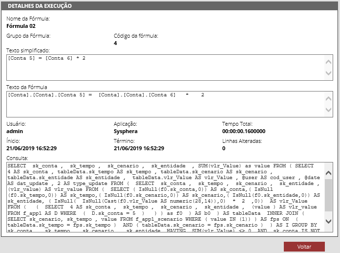
To view more details about a specific execution, click the View Details button on the desired row.
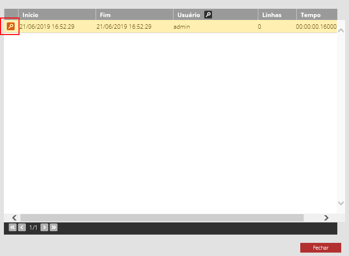
A popup will open with more details of the execution.
It is important to note that if the EnableLogs parameter is not enabled, only the last execution of the formula will be displayed, since the records of previous executions will not be retained. For more details about T6 Planning parameters, refer to the STD Parameters Setup Manual.
¶ 5. Performance
¶ 5.1 Overview
This chapter will cover some important points that will help you achieve maximum performance when using formulas in T6 Planning.
¶ 5.2 Creation
For better formula performance, follow these guidelines:
- Try to write formulas as simply as possible.
- Whenever possible, use the available functions.
- If an expression is repeated across multiple formulas, create a single formula with just that expression and reference it when needed.
- Avoid creating cycles with unnecessary recursions and circular references.
¶ 5.3 Identifying Bottlenecks
To identify formula implementation bottlenecks, identify the form that is showing slowness when saving data and follow the steps below:
-
Clear the formula log table with the following SQL:
TRUNCATE TABLE REP_LOGFORMULA
-
Save data in the form that is showing slowness and check the total save time in seconds.
-
To find the formula save time in seconds, run the following SQL:
SELECT SUM((DATEDIFF(MS,datExecutionStart,datExecutionEnd) / 1000)) as Duration FROM REP_LOGFORMULA
-
To find the total formula execution time in seconds, run the following SQL:
SELECT (DATEDIFF(MS,(SELECT MIN(datExecutionStart) FROM REP_LOGFORMULA),(SELECT MAX(datExecutionEnd) FROM REP_LOGFORMULA)) / 1000) as Duration
-
To find the execution time for each formula in seconds, run the following SQL:
SELECT (DATEDIFF(MS,datExecutionStart,datExecutionEnd) / 1000) as Duration, dscFormulaName FROM REP_LOGFORMULA ORDER BY Duration DESC
-
Divide the value found in step five by the value found in step three and multiply the result by one hundred. This value represents the percentage of time used by formulas. If this percentage is very close to one hundred, check the result from step five to see which formulas are contributing most to the performance problem.
-
Divide the result of step four by step five and multiply the result by one hundred. This value represents the percentage of SQL Server execution time relative to the total formula execution time. If this value is not close to one hundred, the application may be experiencing performance issues.
¶ 5.4 Identifying Problems in Cycles
To help you identify specific problems in cycles, we will describe some occurrences and how to resolve them.
-
Incorrect calculation in a cycle with formula recursion month by month
- Situation: When a form containing a cycle with formula recursion incorrectly calculates a cumulative field, such as the opening balance of a month based on the closing balance of the previous month.
- Solution: Check the formula list to see if any formula is ordered incorrectly — for example, the formula that calculates the opening balance positioned after the one that calculates the closing balance — and if so, reorder it manually, since the system does not reorder formulas that are in cycles. After reordering, the formulas must be re-executed.
- Example: A form for recording monthly revenues and expenses where, at the end of each month, the Closing Balance is calculated based on those entries. This result carries over to the next month, forming the Opening Balance.
When the issue described above occurs, the Opening Balance is calculated incorrectly.
After applying the indicated solution, the Opening Balance calculation will be performed correctly.
-
Incorrect calculation in a cycle with recursion of dependent formulas
- Situation: When a form containing a cycle with formula recursion incorrectly calculates the result of a movement that depends on another, within the same period.
- Solution: Check the movement (Accounts) list to see if the account that depends on the result of another is ordered incorrectly — that is, positioned before it. If so, reorder them manually by placing the account that calculates the first result first, followed by the account that depends on it.
- Example: A form that calculates total monthly expenses by summing fixed expenses with the calculation of weekly expenses. In this case, the calculations are based on movements or Accounts, with weekly expenses being Movement 1 and monthly expenses being Movement 2. When these accounts are incorrectly ordered in reverse position, at the moment the system executes the formulas, only the value of Movement 1 will be calculated. When the formulas are executed a second time, the system will calculate correctly, since in this case the model will resolve itself, as the value of Movement 1 had already been calculated and will then result in the correct calculation of Movement 2.
After applying the solution and correctly ordering Movement 2 after Movement 1, the values will be generated correctly whenever the formulas are executed.
-
Incorrect calculation in a cycle with circular reference
- Situation: When a form calculates different values on each execution of the formula.
- Solution: This type of occurrence is a circular reference, where the calculation of a member's value depends on the result of the parent member — that is, itself. To fix this problem, it is necessary to edit the formula and replace the account with a child member of the resulting account.
- Example: A form that calculates a percentage of the Investment account using the formula: Investment = Revenue + 0.01. In this case, the Revenue account is the parent member of the Investment account, and in this formula, the calculation of Investment depends on the result of the parent member.
After applying the indicated solution and replacing the Investment account with a child member of the Revenue account — such as the Products account, for example — the circular reference will be broken, so that when performing the calculation, the system will be decomposing a parent account into its child accounts.
¶ 5.5 Identifying Other Problems
To verify whether the slowness issue when saving the form is related to formulas:
-
Once you have identified which formulas have performance issues, check if there is a better way to perform the same calculation.
-
Check if there is any intersection interfering with the performance of the calculations. Intersections are occurrences where two formulas or expressions are calculating the same tuple, which must not occur under any circumstances, as this causes recalculation, database overload, and performance degradation.
Whenever necessary, you can access the Order Formulas – Intersections screen; check if there is any intersection created by mistake, such as a duplicate formula, and remove it.
¶ 6. Functions
¶ 6.1 Overview
This chapter will cover the functions available in the application and their purposes.
¶ 6.2 Accessing the Function List
To access the function list in the T6 Planning main menu, go to Modeling -> Formulas.
The Formulas screen will be displayed. Click the Add button in the lower-right corner of the screen.
- On the formula tab, click the Functions button (highlighted on the right side).
The screen displaying the Application Function List will appear. You can navigate through the available functions and view their descriptions. After selecting the desired function, click Ok.
¶ 6.3 Parameter Types
This section presents the Parameter Types used in T6 Planning functions.
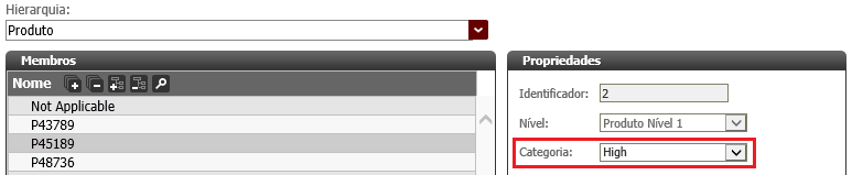
¶ 6.3.1 Attribute
A characteristic applicable to dimension members.
Example:
¶ 6.3.2 Block
A set of elements to be calculated.
Example:
(2 + 3 + 4) = Numeric block
¶ 6.3.3 Column
A column in a database table.
Example:
¶ 6.3.4 Comparator
An expression that compares two values using the operators below, returning true or false.
= equal to
!= not equal to
> greater than
>= greater than or equal to
< less than
<= less than or equal to
Example:
¶ 6.3.5 Conditional
A conditional to be tested. This parameter must be a comparison between two operands. Its syntax must be an operand followed by a comparator followed by an operand.
The operand must be:
- Member, which may or may not have a scope
- Number
- Constant
- A member property
Example:
¶ 6.3.6 Dimension
A dimension is an organized hierarchy of categories, or members. Dimensions represent elements of the company.
Example: Elements can be tangible, such as Employees, Products, or Accounts, or they may represent important views of business data, such as Business Processes, Time, and Scenario.
¶ 6.3.7 Hierarchy
Groupings of different members belonging to the same dimension.
Example:
¶ 6.3.8 Member
A dimension member is a single position or item in a dimension. The set formed by one member from each dimension represents a context in the fact table.
Example:
¶ 6.3.9 Member with Scope
A set of members, one from each dimension.
Example:
¶ 6.3.10 Level
Represents the hierarchical level among members of the same dimension. Being Parent (Level 1), Child (Level 2), Grandchild (Level 3), etc.
Example:
¶ 6.3.11 Number
A mathematical concept for the representation of measure, order, or quantity.
Example:
¶ 6.3.12 Integer
Integers consist of all positive natural numbers, negative numbers, and zero.
Example: Z= {...,−1, −2, −3,−4 ...} or
¶ 6.3.13 Positive Integer
Positive integers consist of positive natural numbers, including zero.
Example: Z+=
¶ 6.3.14 Table
A Database Table.
Example:
¶ 6.3.15 Value
Integer or decimal numbers.
Example:
¶ 7. Available Functions
In this section, the functions available in T6 Planning will be listed, along with their description, syntax, and parameters.
¶ 7.1 Absolute (Abs)
Description:
Returns the absolute value of a number, removing the negative sign if present. The absolute value represents the magnitude of the original number, regardless of its sign. It is used when working with values without considering whether they are positive or negative, such as in analyses of variances, deviations, or financial adjustments.
Syntax:
ABS(Item)
Parameters:
| Name | Description | Parameter Types | Required | Repetitions |
|---|---|---|---|---|
| Item | Value whose absolute value will be calculated | Member, Member with Scope, Block | Yes | No |
Click here to view an example:
| Formula | Description | Result |
|---|---|---|
| ABS([Variação Orçamento]) | Absolute value of 500.00 | 500.00 |
| ABS([Variação Orçamento]) | Absolute value of -300.00 | 300.00 |
Result Description: The function returns the absolute value of the provided number. For a negative variance of R$ -300.00, the function returns R$ 300.00, disregarding the negative sign and enabling magnitude comparisons between periods.
¶ 7.2 Adjust
Description:
Performs a percentage adjustment on a base value, applying a positive or negative variation. The formula used internally is Result = Value × (1 + Percentage / 100). It is widely used in planning to simulate salary adjustments, price increases, or budget corrections over time.
Syntax:
Adjust(Item, Percentage, Attribute)
Parameters:
| Name | Description | Parameter Types | Required | Repetitions |
|---|---|---|---|---|
| Item | Base value to be adjusted | Member, Member with Scope, Block | Yes | No |
| Percentage | Adjustment percentage to be applied | Member, Member with Scope | Yes | No |
| Attribute | Dimension attribute for segmentation of the adjustment | Dimension, Attribute, Value | No | Yes |
Click here to view an example:
| Data | Description |
|---|---|
| 5,000.00 | Current salary (Item) |
| 8% | Adjustment percentage (Percentage) |
| Formula | Description | Result |
|---|---|---|
| [Salário Reajustado] = Adjust([Salário], [% Reajuste]) | Applies an 8% adjustment to the current salary | 5,400.00 |
Result Description: The salary of R$ 5,000.00 is multiplied by (1 + 8/100) = 1.08, resulting in R$ 5,400.00. For negative adjustments (e.g., -5%), the value would be multiplied by 0.95.
¶ 7.3 Between
Description:
Returns the sum of a member's values within a range of periods defined by a start date and an end date. Only the periods between the two dates (inclusive) are considered in the calculation. It is used to calculate totals within specific time windows, such as the total salaries paid between an employee's hire and termination date.
Syntax:
Between(Value, StartDate, EndDate)
Parameters:
| Name | Description | Parameter Types | Required | Repetitions |
|---|---|---|---|---|
| Value | Value to be summed over the period range | Member, Member with Scope | Yes | No |
| StartDate | Start date or period of the range | Member, Member with Scope | Yes | No |
| EndDate | End date or period of the range | Member, Member with Scope | Yes | No |
Click here to view an example:
| Data | Description |
|---|---|
| 3,000.00 | Monthly salary (Value) |
| Jan/24 | Hire date (StartDate) |
| May/24 | Termination date (EndDate) |
| Formula | Description | Result |
|---|---|---|
| Between([Salário Mensal], [Tempo].[2024].[Janeiro/24], [Tempo].[2024].[Maio/24]) | Sums the monthly salary across the 5 months between January and May 2024 | 15,000.00 |
Result Description: The function sums the salary of R$ 3,000.00 for each of the 5 months in the range (Jan, Feb, Mar, Apr, May), returning a total of R$ 15,000.00. Periods outside the specified range are not considered.
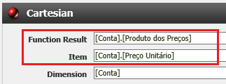
¶ 7.4 Cartesian
Description:
Creates a Cartesian product between an item and one or more specified dimensions, distributing or replicating the value across all possible combinations of members from the provided dimensions. It is used when you want to propagate a base value to all dimension combinations, such as distributing a total budget across all combinations of product and scenario.
Syntax:
Cartesian(Item, Dimension1, Dimension2, ..., DimensionN)
Parameters:
| Name | Description | Parameter Types | Required | Repetitions |
|---|---|---|---|---|
| Item | Value to be distributed across the Cartesian product | Member, Member with Scope, Block | Yes | No |
| Dimension | Dimension whose members will participate in the Cartesian product | Dimension | Yes | Yes |
Click here to view an example:
| Sample Data | ||
|---|---|---|
| Product | Scenario | Sales Value |
| Smartphone | Budgeted | R$ 10,000.00 |
| Smartphone | Actual | R$ 10,000.00 |
| TV | Budgeted | R$ 10,000.00 |
| TV | Actual | R$ 10,000.00 |
| Formula | Description | Result |
|---|---|---|
| [Vendas Total] = Cartesian([Vendas Total], [Produto], [Cenário]) | Distributes the value of [Vendas Total] to each combination of members from the Product and Scenario dimensions | R$ 10,000.00 replicated across all 4 combinations |
Result Description: The value of R$ 10,000.00 is replicated for the four combinations generated by the Cartesian product between Product and Scenario: Smartphone/Budgeted, Smartphone/Actual, TV/Budgeted, and TV/Actual.
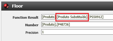
¶ 7.5 Ceiling
Description:
Rounds a number upward, returning the smallest integer that is greater than or equal to the specified value. Optionally, a decimal precision can be provided to control the rounding level. It is used in provisions, quantity, and budget calculations where fractional values must always be rounded up for safety.
Syntax:
Ceiling(Number, Precision)
Parameters:
| Name | Description | Parameter Types | Required | Repetitions |
|---|---|---|---|---|
| Number | Number to be rounded upward | Member, Member with Scope, Block | Yes | No |
| Precision | Decimal precision for rounding | Integer | No | No |
Click here to view an example:
| Formula | Description | Result |
|---|---|---|
| Ceiling([Qtd Unidades]) | Rounds 2.3 units upward without precision | 3 |
| Ceiling([Custo Unitário], 2) | Rounds 15.234 upward with 2 decimal places | 15.24 |
| Ceiling([Provisão], 0) | Rounds 1,234.70 upward with no decimal places | 1,235 |
Result Description: The function ensures that fractional values are always rounded upward. With precision 2, the value 15.234 becomes 15.24. Without a defined precision, rounding is performed to the next higher integer.
¶ 7.6 CGrow
Description:
Calculates the compound growth of a value over periods, applying a percentage growth rate to the accumulated value from the previous period and adding a fixed increment. The formula used is: Result = Previous Value × (1 + Rate/100) + Increment. It is used to project growth of revenues, salaries, or any quantity that grows in a compound manner over time.
Syntax:
CGrow(Start, Grow, %GrowRate)
Parameters:
| Name | Description | Parameter Types | Required | Repetitions |
|---|---|---|---|---|
| Start | Initial base value for the first period | Member, Member with Scope | Yes | No |
| Grow | Fixed increment added each period | Member, Member with Scope | Yes | No |
| %GrowRate | Compound growth percentage rate | Member, Member with Scope | Yes | No |
Click here to view an example:
| Data | Description |
|---|---|
| 1,000.00 | Initial value (Start) |
| 200.00 | Fixed increment per period (Grow) |
| 10% | Compound growth rate (%GrowRate) |
| Formula | Description |
|---|---|
| CGrow([Receita Base], [Incremento Mensal], [% Crescimento]) | Calculates the accumulated value applying compound growth and fixed increment each period |
| Account | Period 1 | Period 2 | Period 3 | Period 4 |
|---|---|---|---|---|
| Initial Value (Start) | 1,000.00 | 1,320.00 | 1,682.00 | 2,090.20 |
| Increment (Grow) | 200.00 | 200.00 | 200.00 | 200.00 |
| Rate (%GrowRate) | 10% | 10% | 10% | 10% |
| Period Result | 1,320.00 | 1,682.00 | 2,090.20 | 2,559.22 |
Result Description: Each period, compound growth is applied to the previous accumulated result, adding the fixed increment. The growth is compound — each period grows on a value that is already larger than the previous one.
¶ 7.7 Closing
Description:
Calculates the closing balance based on the opening balance, summing inflows and subtracting outflows. Implements the classic accounting formula: Closing Balance = Opening Balance + Inflows - Outflows. It is essential in financial and accounting contexts for calculating closing balances of accounts, inventory, or cash flow over time.
Syntax:
Closing(Opening, In, Out)
Parameters:
| Name | Description | Parameter Types | Required | Repetitions |
|---|---|---|---|---|
| Opening | Opening balance for the period | Member, Member with Scope | Yes | No |
| In | Inflow movements | Member, Member with Scope | Yes | Yes |
| Out | Outflow movements | Member, Member with Scope | No | Yes |
Click here to view an example:
| Data | Description |
|---|---|
| 1,000.00 | Opening balance (Opening) |
| 500.00 | Inflow movements (In) |
| 200.00 | Outflow movements (Out) |
| Formula | Description | Result |
|---|---|---|
| [Saldo Final] = Closing([Saldo Inicial], [Entradas], [Saídas]) | Calculates the closing balance by adding inflows and subtracting outflows from the opening balance | 1,300.00 |
| Account | Period 1 |
|---|---|
| Opening Balance (Opening) | 1,000.00 |
| Inflow Movements (In) | 500.00 |
| Outflow Movements (Out) | 200.00 |
| Closing Balance | 1,300.00 |
Result Description: The closing balance of R$ 1,300.00 is obtained by adding the opening balance (R$ 1,000.00) to inflows (R$ 500.00) and subtracting outflows (R$ 200.00). Multiple inflow and outflow parameters can be provided; all are summed or subtracted respectively.
¶ 7.8 ClosingVariance
Description:
Calculates the closing balance with percentage variance — a more sophisticated version of the Closing function. In addition to direct inflows and outflows, it applies percentage variations on the opening balance and an amortization divisor. The formula is: Closing Balance = Opening + (Opening × In%) - (Opening × Out%) - (Opening ÷ Divider) + Inflows - Outflows. It is used to model loan balances, provisioned remuneration, and combined depreciation.
Syntax:
ClosingVariance(Opening, OpeningIn%, OpeningOut%, DividerOutput, In, Out)
Parameters:
| Name | Description | Parameter Types | Required | Repetitions |
|---|---|---|---|---|
| Opening | Opening balance for the period | Member, Member with Scope | Yes | No |
| Opening In % | Positive variance percentage applied to the opening balance | Member, Member with Scope, Number | Yes | No |
| Opening Out % | Negative variance percentage applied to the opening balance | Member, Member with Scope, Number | Yes | No |
| Divider Output | Divisor applied to the opening balance for amortization or reduction | Member, Member with Scope, Number | Yes | No |
| In | Additional inflow movements | Member, Member with Scope | Yes | Yes |
| Out | Additional outflow movements | Member, Member with Scope | No | Yes |
Click here to view an example:
| Data | Description |
|---|---|
| 10,000.00 | Opening balance (Opening) |
| 2% | Interest rate on balance (Opening In %) |
| 1% | Service fee percentage (Opening Out %) |
| 24 | Amortization term in months (Divider Output) |
| 500.00 | Additional contributions (In) |
| 200.00 | Withdrawals (Out) |
| Formula | Description | Result |
|---|---|---|
| [Saldo Final] = ClosingVariance([Saldo], [% Juros], [% Taxa], [Prazo], [Aportes], [Retiradas]) | Calculates the closing balance applying interest, fee, and amortization on the opening balance | 10,383.33 |
Result Description: The balance of R$ 10,000.00 receives 2% interest (+R$ 200.00), deducts the 1% service fee (-R$ 100.00), deducts the amortization installment (10,000 ÷ 24 = -R$ 416.67), adds contributions (+R$ 500.00), and subtracts withdrawals (-R$ 200.00), resulting in R$ 9,983.33.
¶ 7.9 CumAdjust
Description:
Accumulates a value over periods applying compound operations: adds an increment, multiplies by a rate, and adds a post-multiplication increment. Internally uses a recursive CTE (Common Table Expression) to ensure correct propagation of the accumulated value between periods. The Restart parameter allows the accumulation to be restarted from a specific value in any period.
Syntax:
CumAdjust(Increment, Multiplier%, IncrementAfterMultiplier, Restart)
Parameters:
| Name | Description | Parameter Types | Required | Repetitions |
|---|---|---|---|---|
| Increment | Increment value added to the accumulation each period | Member, Member with Scope | Yes | No |
| Multiplier % | Multiplier percentage applied to the accumulated value | Member, Member with Scope, Number | No | No |
| Increment After Multiplier | Increment added after multiplication | Member, Member with Scope, Number | No | No |
| Restart | Value that restarts the accumulation in the next period | Member, Member with Scope | No | No |
Click here to view examples:
Result with Increment
| Data | Description | |
|---|---|---|
| 100 | Accumulated (previous period value, calculated by the formula itself) | |
| 100 | Increment | |
| Formula | Description | Result |
| [Acumulado] = CumAdjust([Increment]) | Adds the increment to the previous period's accumulated value | 200 |
Result with Increment and Multiplier
| Data | Description | |
|---|---|---|
| 100 | Accumulated (previous period value) | |
| 100 | Increment | |
| 10% | Multiplier % | |
| Formula | Description | Result |
| [Acumulado] = CumAdjust([Increment], [Multiplier]) | Adds the increment and applies the multiplier to the total | 220 |
Result with Increment After Multiplication
| Data | Description | |
|---|---|---|
| 100 | Accumulated (previous period value) | |
| 100 | Increment | |
| 10% | Multiplier % | |
| 100 | Increment after multiplication | |
| Formula | Description | Result |
| [Acumulado] = CumAdjust([Increment], [Multiplier], [IncrementAfterMultiplier]) | Adds the increment, applies the multiplier, and adds the post-multiplication increment | 320 |
Result with Restart
| Data | Description | |
|---|---|---|
| 100 | Accumulated (previous period value) | |
| 100 | Increment | |
| 10% | Multiplier % | |
| 100 | Increment after multiplication | |
| 0 | Restart | |
| Formula | Description | Result |
| [Acumulado] = CumAdjust([Increment], [Multiplier %], [IncrementAfterMultiplier], [Restart]) | Calculates the accumulated value and restarts in the next period with the Restart value | 320 (current), 0 (next) |
Restart application example:
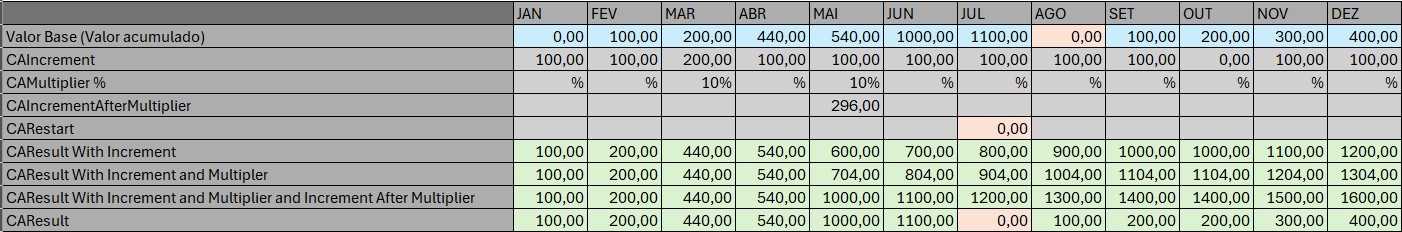
Result Description: The Restart parameter replaces the accumulated value in the current period, causing the next period to start with the value specified in Restart instead of the calculated value.
¶ 7.10 Cumulate
Description:
Progressively accumulates a member's values over periods, returning the sum of all values from the first period through the current period. Each period, the result is the sum of all previous period values plus the current period value. It is used to calculate year-to-date (YTD) totals, accumulated sales, or any metric that needs to be summed progressively.
Syntax:
Cumulate(Value[, TipoCalculo])
Parameters:
| Name | Description | Parameter Types | Required | Repetitions |
|---|---|---|---|---|
| Value | Value to be accumulated period by period | Member, Member with Scope | Yes | No |
| TipoCalculo | Calculation type: "normal" (default), "window", or "windowfull" |
Value | No | No |
Click here to view an example:
| Data | Description |
|---|---|
| Jan: 100.00 | January Revenue (Value) |
| Feb: 150.00 | February Revenue |
| Mar: 120.00 | March Revenue |
| Formula | Period | Accumulated Result |
|---|---|---|
| Cumulate([Receita Mensal]) | January | 100.00 |
| Cumulate([Receita Mensal]) | February | 250.00 |
| Cumulate([Receita Mensal]) | March | 370.00 |
Result Description: The function sums all values from the beginning through the current period. In March, the accumulated total of R$ 370.00 represents the sum of January (100.00) + February (150.00) + March (120.00).
¶ 7.11 Delay
Description:
Distributes an input value across multiple future periods, applying a specific percentage for each lag period. Each %Period parameter corresponds to a period offset relative to the original transaction period. It is widely used to model default rates, installment sales receipts, or payments distributed over time.
Syntax:
Delay(Input, %Period1, %Period2, ..., %PeriodN)
Parameters:
| Name | Description | Parameter Types | Required | Repetitions |
|---|---|---|---|---|
| Input | Total value to be distributed across periods | Member, Member with Scope | Yes | No |
| % Period | Percentage to be applied in each lag period | Member, Member with Scope, Number | Yes | Yes |
Click here to view an example:
| Data | Description |
|---|---|
| 10,000.00 | Sale value (Input) |
| 40% | Receipt in the month of the sale (1st %Period) |
| 35% | Receipt in the following month (2nd %Period) |
| 25% | Receipt in 2 months (3rd %Period) |
| Formula | Period | Result |
|---|---|---|
| Delay([Vendas], [% Mês 0], [% Mês 1], [% Mês 2]) | January (month of sale) | 4,000.00 |
| Delay([Vendas], [% Mês 0], [% Mês 1], [% Mês 2]) | February | 3,500.00 |
| Delay([Vendas], [% Mês 0], [% Mês 1], [% Mês 2]) | March | 2,500.00 |
Result Description: The sale value of R$ 10,000.00 is distributed over 3 months: 40% (R$ 4,000.00) received in the month of the sale, 35% (R$ 3,500.00) in the following month, and 25% (R$ 2,500.00) two months later. The sum of percentages must total 100%.
¶ 7.12 Depr
Description:
Calculates the straight-line depreciation of an asset based on its value and useful life. The formula is: Depreciation = Asset Value ÷ Useful Life. Straight-line depreciation distributes the loss of value evenly across each period. It is used in financial planning to provision for the depreciation of fixed assets such as equipment, vehicles, and facilities.
Syntax:
Depr(Capitalization, Life)
Parameters:
| Name | Description | Parameter Types | Required | Repetitions |
|---|---|---|---|---|
| Capitalization | Value of the asset to be depreciated | Member, Member with Scope | Yes | No |
| Life | Useful life of the asset (in periods) | Member, Member with Scope | Yes | No |
Click here to view an example:
| Data | Description |
|---|---|
| 60,000.00 | Vehicle value (Capitalization) |
| 60 | Useful life in months (Life) |
| Formula | Description | Result |
|---|---|---|
| Depr([Valor Veículo], [Vida Útil]) | Calculates the monthly straight-line depreciation of the vehicle | 1,000.00 per month |
Result Description: The vehicle worth R$ 60,000.00 is depreciated linearly over 60 months, generating a depreciation expense of R$ 1,000.00 per month. At the end of 60 months, the total depreciated amount equals the original asset value.
¶ 7.13 Descendants
Description:
Returns the values of the descendant members of a member in the hierarchy, excluding the value of the specified member itself. That is, it returns only the sum of child members and all lower levels. It is used when you want to obtain the breakdown of a hierarchical total without including the aggregated value at the parent level, such as getting sales by region without including the grand total.
Syntax:
Descendants(Member)
Parameters:
| Name | Description | Parameter Types | Required | Repetitions |
|---|---|---|---|---|
| Member | Parent member whose descendants will be returned | Member, Member with Scope | Yes | No |
Click here to view an example:
| Data | Description |
|---|---|
| Total Sales: 300,000.00 | Parent member (not included in the result) |
| South: 80,000.00 | Descendant 1 |
| Southeast: 120,000.00 | Descendant 2 |
| North: 100,000.00 | Descendant 3 |
| Formula | Description | Result |
|---|---|---|
| Descendants([Total Vendas]) | Returns the values of each descendant region, without including the total | South: 80,000, Southeast: 120,000, North: 100,000 |
Result Description: The function returns the values of the three regions (South, Southeast, and North) without including the aggregated value of "Total Sales". Useful for detailing individual components of a hierarchy without risk of duplicating the total.
¶ 7.14 DiffFirstValue
Description:
Calculates the difference between the current member's value and the first value found in the hierarchy, considering vertical (parent level) and horizontal (period) offsets. It is used for comparative analyses in hierarchical structures, such as calculating the variance of each month relative to the first month of the year or each product relative to the base product in the hierarchy.
Syntax:
DiffFirstValue(Item, Parent, Lag, Dimension)
Parameters:
| Name | Description | Parameter Types | Required | Repetitions |
|---|---|---|---|---|
| Item | Value of the member for which the difference is calculated | Member, Member with Scope, Block | Yes | No |
| Parent | Vertical offset in the hierarchy (parent level) | Positive Integer | Yes | No |
| Lag | Horizontal offset (periods) | Integer | Yes | No |
| Dimension | Dimension in which the first value will be searched | Dimension, Hierarchy | No | No |
Click here to view an example:
| Data | Description |
|---|---|
| Jan/24: 100,000.00 | January Revenue (first value in Time hierarchy) |
| Feb/24: 120,000.00 | February Revenue |
| Mar/24: 140,000.00 | March Revenue |
| Formula | Period | Result |
|---|---|---|
| DiffFirstValue([Receita], 0, 0, [Tempo]) | January | 0 |
| DiffFirstValue([Receita], 0, 0, [Tempo]) | February | 20,000.00 |
| DiffFirstValue([Receita], 0, 0, [Tempo]) | March | 40,000.00 |
Result Description: The function subtracts the first value in the hierarchy (January = R$ 100,000.00) from the value of each period. February shows a variance of +R$ 20,000.00 and March of +R$ 40,000.00 relative to the first month.
¶ 7.15 DiffLastValue
Description:
Calculates the difference between the current member's value and the last value found in the hierarchy, considering vertical (parent level) and horizontal (period) offsets. It is used for variance analyses relative to closure, such as comparing each month with the year-end result or identifying how much each item is below or above the last reference value.
Syntax:
DiffLastValue(Item, Parent, Lag, Dimension)
Parameters:
| Name | Description | Parameter Types | Required | Repetitions |
|---|---|---|---|---|
| Item | Value of the member for which the difference is calculated | Member, Member with Scope, Block | Yes | No |
| Parent | Vertical offset in the hierarchy (parent level) | Positive Integer | Yes | No |
| Lag | Horizontal offset (periods) | Integer | Yes | No |
| Dimension | Dimension in which the last value will be searched | Dimension, Hierarchy | No | No |
Click here to view an example:
| Data | Description |
|---|---|
| Jan/24: 100,000.00 | January Revenue |
| Feb/24: 120,000.00 | February Revenue |
| Mar/24: 140,000.00 | March Revenue (last value in Time hierarchy) |
| Formula | Period | Result |
|---|---|---|
| DiffLastValue([Receita], 0, 0, [Tempo]) | January | -40,000.00 |
| DiffLastValue([Receita], 0, 0, [Tempo]) | February | -20,000.00 |
| DiffLastValue([Receita], 0, 0, [Tempo]) | March | 0 |
Result Description: The function subtracts the last value in the hierarchy (March = R$ 140,000.00) from the value of each period. January shows -R$ 40,000.00 and February -R$ 20,000.00 relative to the closing month.
¶ 7.16 DiffPercent
Description:
Calculates the percentage variance between the current period value and the value of a previous period, based on a configurable step. The formula is: (Current Value - Previous Value) / Previous Value × 100. The Step parameter defines how many lag periods to consider (default: 1). It is used to calculate percentage growth month over month, quarter over quarter, or between any two periods.
Syntax:
DiffPercent(Value, Step)
Parameters:
| Name | Description | Parameter Types | Required | Repetitions |
|---|---|---|---|---|
| Value | Base value for calculating the percentage variance | Member, Member with Scope | Yes | No |
| Step | Number of lag periods for comparison (default: 1) | Member, Member with Scope, Integer | No | No |
Click here to view an example:
| Data | Description |
|---|---|
| Jan/24: 100,000.00 | January Revenue |
| Feb/24: 120,000.00 | February Revenue |
| Mar/24: 114,000.00 | March Revenue |
| Formula | Period | Result |
|---|---|---|
| DiffPercent([Receita Mensal], 1) | January | - (no previous period) |
| DiffPercent([Receita Mensal], 1) | February | 20.00% |
| DiffPercent([Receita Mensal], 1) | March | -5.00% |
Result Description: The function returns the percentage variance relative to the previous period. February grew 20% over January ((120,000 - 100,000) / 100,000 × 100). March fell 5% from February ((114,000 - 120,000) / 120,000 × 100). For the first period there is no calculation as there is no prior reference period.
¶ 7.17 DiffProportion
Description:
Calculates the proportional difference between the current period value and a previous period value, using the formula (current - previous) / current. Useful for relative growth analyses, identifying the percentage variance of a value relative to the reference period.
The Step parameter controls how many periods back the comparison is made. When omitted, the default value is 1 (immediately previous period).
Syntax:
DiffProportion(Value, Step)
Parameters:
| Name | Description | Parameter Types | Required | Repetitions |
|---|---|---|---|---|
| Value | Base value for the proportional difference calculation | Member, Member with Scope, Block | Yes | No |
| Step | Number of periods of distance for the comparison | Integer | No | No |
Click here to view an example:
| Period | Monthly Revenue |
|---|---|
| January | R$ 100,000 |
| February | R$ 120,000 |
| March | R$ 150,000 |
| Formula | Description | Result |
|---|---|---|
| DiffProportion([Receita Mensal], 1) | Calculates the proportional difference between the current month and the previous month. | February: 0.1667 ((120k - 100k) / 120k), March: 0.2 ((150k - 120k) / 150k) |
Result Description: The function returns the proportional variance between periods. For the first period (January) there is no result, as there is no previous period for comparison.
¶ 7.18 DiffValue
Description:
Calculates the absolute value difference between the current period and a previous period, using the formula current - previous. Useful for temporal variance analyses, identifying the absolute growth or decline between consecutive periods or with custom intervals.
The Step parameter controls how many periods back the comparison is made. When omitted, the default value is 1 (immediately previous period).
Syntax:
DiffValue(Value, Step)
Parameters:
| Name | Description | Parameter Types | Required | Repetitions |
|---|---|---|---|---|
| Value | Base value for the absolute difference calculation | Member, Member with Scope, Block | Yes | No |
| Step | Number of periods of distance for the comparison | Integer | No | No |
Click here to view an example:
| Period | Monthly Revenue |
|---|---|
| January | R$ 100,000 |
| February | R$ 120,000 |
| March | R$ 150,000 |
| Formula | Description | Result |
|---|---|---|
| DiffValue([Receita Mensal], 1) | Calculates the value difference between the current month and the previous month. | February: R$ 20,000 (120k - 100k), March: R$ 30,000 (150k - 120k) |
Result Description: The function returns the absolute variance between periods. For the first period (January) there is no result, as there is no previous period for comparison.
¶ 7.19 Expand
Description:
Expands an item from a hierarchical level to child members within a specified level range, using INNER JOIN on the dimension hierarchy tables. Allows distributing a value from a higher level to all its descendants between the start level and the end level.
Multiple dimension/level pairs can be specified to work with different dimensions simultaneously.
Syntax:
Expand(Item, Level Start, Level End)
Parameters:
| Name | Description | Parameter Types | Required | Repetitions |
|---|---|---|---|---|
| Item | Item to be expanded in the hierarchy | Member, Member with Scope, Block | Yes | No |
| Level Start | Dimension and start level of the expansion | Dimension, Level | Yes | Yes |
| Level End | Dimension and end level of the expansion | Dimension, Level | Yes | Yes |
Click here to view an example:
| Level | Members |
|---|---|
| Region | South, Southeast |
| State | Paraná, São Paulo |
| City | Curitiba, Londrina, Campinas, São Paulo (SP) |
| Formula | Description | Result |
|---|---|---|
| Expand([Vendas], [Entidade].[Região], [Entidade].[Cidade]) | Expands the value of [Vendas] from the Region level to the City level, distributing to each corresponding city. | South → Curitiba: R$ 300, Londrina: R$ 200; Southeast → Campinas: R$ 700, São Paulo (SP): R$ 500 |
Result Description: The function traverses the hierarchy levels of the Entity dimension, from the Region level to the City level, returning the detailed values of each descendant member.
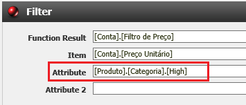
¶ 7.20 Filter
Description:
Filters a block of values by the attributes of dimension members, using INNER JOIN on the attribute tables. Returns only the values whose members satisfy the specified attribute conditions.
Multiple filters can be applied simultaneously, combining different attributes from different dimensions to refine the returned dataset.
Syntax:
Filter(Item, Attribute)
Parameters:
| Name | Description | Parameter Types | Required | Repetitions |
|---|---|---|---|---|
| Item | Data block to be filtered | Block | Yes | No |
| Attribute | Dimension, attribute, and value by which to filter members | Dimension, Attribute, Value | Yes | Yes |
Click here to view an example:
| Product | Category | Sales |
|---|---|---|
| Smartphone | Electronics | R$ 10,000 |
| TV | Electronics | R$ 15,000 |
| Refrigerator | Appliances | R$ 8,000 |
| Washing Machine | Appliances | R$ 7,000 |
| Formula | Description | Result |
|---|---|---|
| Filter([Vendas], [Produto].[Categoria].[Eletrônicos]) | Filters the [Vendas] block to include only products with Category attribute equal to Electronics. | Smartphone: R$ 10,000, TV: R$ 15,000 |
| Filter([Vendas], [Produto].[Categoria].[Eletrodomésticos]) | Filters the [Vendas] block to include only products with Category attribute equal to Appliances. | Refrigerator: R$ 8,000, Washing Machine: R$ 7,000 |
Result Description: The Filter function traverses the members of the Product dimension and returns only the values of members whose Category attribute matches the specified value.
Description:
Returns the first value of an item within a hierarchy, considering vertical (how many levels up in the hierarchy) and horizontal (how many periods of offset) displacements. Useful for retrieving the initial value of a sequence within a hierarchical group.
The Dimension parameter allows explicitly specifying the dimension to navigate; when omitted, the default time dimension is used.
Syntax:
FirstValue(Item, Parent, Lag, Dimension)
Parameters:
| Name | Description | Parameter Types | Required | Repetitions |
|---|---|---|---|---|
| Item | Item from which to retrieve the first value | Member, Member with Scope, Block | Yes | No |
| Parent | Vertical offset in the hierarchy (number of levels up) | Positive Integer | Yes | No |
| Lag | Horizontal offset (period offset) | Integer | Yes | No |
| Dimension | Dimension and hierarchy for navigation | Dimension, Hierarchy | No | Yes |
Click here to view an example:
| Semester | Quarter | Month | Revenue |
|---|---|---|---|
| 1H/25 | Q1/25 | January/25 | R$ 50,000 |
| 1H/25 | Q1/25 | February/25 | R$ 60,000 |
| 1H/25 | Q1/25 | March/25 | R$ 55,000 |
| 1H/25 | Q2/25 | April/25 | R$ 70,000 |
| Formula | Description | Result |
|---|---|---|
| FirstValue([Receita], 1, 0, [Tempo].[Mensal]) | Returns the first month of each quarter (1 level up = Quarter), without horizontal offset. | Q1/25: R$ 50,000 (January), Q2/25: R$ 70,000 (April) |
Result Description: The function identifies the first value within the group determined by the parent level (Quarter), returning the Revenue of the first month of each quarter.
¶ 7.22 Floor
Description:
Rounds a number downward, returning the largest integer (or with specified precision) that is less than or equal to the provided value. Uses the SQL FLOOR() function internally.
Unlike conventional rounding, Floor always rounds toward negative infinity, regardless of the decimal part of the number. The Precision parameter defines the number of decimal places to retain; when omitted, rounds to the nearest integer below.
Syntax:
Floor(Number, Precision)
Parameters:
| Name | Description | Parameter Types | Required | Repetitions |
|---|---|---|---|---|
| Number | Numeric value to be rounded downward | Member, Member with Scope, Block | Yes | No |
| Precision | Number of decimal places to preserve | Integer | No | No |
Click here to view an example:
| Product | Calculated Price |
|---|---|
| Product A | R$ 43.14 |
| Product B | R$ 18.89 |
| Formula | Description | Result |
|---|---|---|
| Floor([Preço Calculado], 1) | Rounds down with 1 decimal place. | Product A: R$ 43.10; Product B: R$ 18.80 |
| Floor([Preço Calculado]) | Rounds down without decimal places. | Product A: R$ 43.00; Product B: R$ 18.00 |
Result Description: The Floor function ensures that values are always rounded downward, never exceeding the original value. Useful for pricing calculations and financial rules that require conservative values.
¶ 7.23 GetApplicationData
Description:
Reads and integrates data from another application (planning cube) into the current formula. Allows referencing calculated or stored values in a different cube, automatically mapping dimensions between applications.
If the target application has the same dimension ID as the source application, the data is brought over maintaining the mapping. Dimensions present in the target application but absent in the source are populated with -1 (not applicable).
Syntax:
GetApplicationData(Aplicação, Membro)
Parameters:
| Name | Description | Parameter Types | Required | Repetitions |
|---|---|---|---|---|
| Aplicação | Source application for the data | Application | Yes | No |
| Membro | Member of the source application that contains the data | Member, Member with Scope | Yes | Yes |
Click here to view an example:
| Data | Description |
|---|---|
| Planejamento Comercial | Source application |
| [Conta].[Receita Bruta] | Member of the Account dimension in the source application |
| Formula | Description | Result |
|---|---|---|
| [Conta].[Receita Consolidada] = GetApplicationData([Planejamento Comercial], [Conta].[Receita Bruta]) | Loads the values of the Receita Bruta member from the Planejamento Comercial application into the Receita Consolidada member in the current application. | The values of Receita Bruta are copied to Receita Consolidada, with dimensions mapped automatically. |
If the target application has the same dimension ID as the application set in the "Application" parameter, the data will be brought over and kept identical. If the dimension ID exists in the target application but not in the source application, it will be set to -1 (not applicable).
¶ 7.24 GetDataTableData
Description:
Reads and integrates data stored in a Data Table into the current formula. Allows querying external or reference data without needing to store it directly in the cube's dimensional structures.
If the data table has a column linked to a dimension, the system performs the mapping automatically. Dimensions not specified in the scope are treated as "Not applicable".
Syntax:
GetDataTableData(Tabela, Coluna)
Parameters:
| Name | Description | Parameter Types | Required | Repetitions |
|---|---|---|---|---|
| Tabela | Source data table | Table | Yes | No |
| Coluna | Column in the data table that contains the values or the dimensional mapping | Column | No | Yes |
Click here to view an example:
| Data Table | Column | Value |
|---|---|---|
| Total de Itens Vendidos | Valor | 500 |
| Formula | Description | Result |
|---|---|---|
| ([Conta].[Produtos], [Tempo].[Março/25], [Cenário].[Planejado]) = GetDataTableData([Total de Itens Vendidos], [Valor]) | Loads the value from the Valor column of the Total de Itens Vendidos table for the defined scope. | Loads the value 500 to the Products member for March/25, Planned scenario. |
For dimensions not specified in the scope, the system assumes Not applicable.
If the data table has a linked column (link) to a dimension, it is not necessary to specify that dimension in the scope — the system will perform the mapping automatically.
Example formula using a link to the time dimension: ([Produtos], [Cenário].[Planejado]) = GetDataTableData([Total de Itens Vendidos]). In this example, the data table has a column linked to the time dimension.
¶ 7.25 Group
Description:
Aggregates values from a block to a higher hierarchical level of the dimension, using SUM and INNER JOIN on the level tables. The function moves up the hierarchy, consolidating child member values into their respective parent members at the specified level.
Dimension and level pairs can be repeated to group by multiple dimensions simultaneously.
Syntax:
Group(Item, Level)
Parameters:
| Name | Description | Parameter Types | Required | Repetitions |
|---|---|---|---|---|
| Item | Data block to be grouped | Block | Yes | No |
| Level | Dimension and target level for grouping | Dimension, Level | Yes | Yes |
Click here to view an example:
| City | State | Country | Sales |
|---|---|---|---|
| Ubatuba | São Paulo | Brazil | R$ 10,000 |
| Campinas | São Paulo | Brazil | R$ 8,000 |
| Niterói | Rio de Janeiro | Brazil | R$ 12,000 |
| Formula | Result | |
|---|---|---|
| Group([Vendas], [Entidade].[País]) | Country | Total |
| Brazil | R$ 30,000 |
| Formula | Result | |
|---|---|---|
| Group([Vendas], [Entidade].[Estado]) | State | Total |
| São Paulo | R$ 18,000 | |
| Rio de Janeiro | R$ 12,000 |
Result Description: The Group function consolidates the sales values by different hierarchical levels of the Entity dimension, summing the child member values at the specified level.
¶ 7.26 HasValue
Description:
Checks whether an item has a recorded value (not null), returning 1 if the value exists and 0 otherwise. Uses LEFT JOIN and CASE internally to identify the presence of data in the cube.
Useful for identifying the presence of data in analyses, especially when filtering or counting cells with meaningful values in reports.
Syntax:
HasValue(Valor)
Parameters:
| Name | Description | Parameter Types | Required | Repetitions |
|---|---|---|---|---|
| Valor | Item to be checked for the existence of a value | Member, Member with Scope, Block | Yes | No |
Click here to view an example:
| Product | January/25 | February/25 | March/25 |
|---|---|---|---|
| Product A | R$ 500 | R$ 700 | - (NULL) |
| Product B | - (NULL) | - (NULL) | - (NULL) |
| Product C | R$ 300 | - (NULL) | R$ 900 |
| Formula | Product | January/25 | February/25 | March/25 |
|---|---|---|---|---|
| HasValue([Vendas]) | Product A | 1 | 1 | 0 |
| Product B | 0 | 0 | 0 | |
| Product C | 1 | 0 | 1 |
Result Description: The HasValue function returns 1 for cells that have recorded values and 0 for null cells. Useful for identifying the presence of data and building conditional formulas based on the existence of values.
¶ 7.27 IIF
Description:
A conditional function that evaluates a logical expression and returns one value if the condition is true or another value if the condition is false. Multiple conditions can be chained using AND logic.
The condition is formed by three elements: the left operand, a comparator, and the right operand. When the Else parameter is omitted, the function returns null for the false case.
Syntax:
IIF(Condition Left Comparator Condition Right, Then, Else)
Parameters:
| Name | Description | Parameter Types | Required | Repetitions |
|---|---|---|---|---|
| Condition Left | Left operand of the condition | Member, Member with Scope, Number | Yes | No |
| Comparador | Comparison operator (=, <>, <, >, <=, >=) | Comparator | Yes | No |
| Condition Right | Right operand of the condition | Member, Member with Scope, Number | Yes | No |
| Then | Value returned when the condition is true | Member, Member with Scope, Number, Conditional | Yes | No |
| Else | Value returned when the condition is false | Member, Member with Scope, Number, Conditional | No | No |
Comments: Not all possible combinations between operands and comparators are valid. Below is the list of valid combinations:
Click to expand the possible combinations
- Member, Less Than or Equal, Member- Member, Greater Than or Equal, Member
- Member, Not Equal, Member
- Member, Equal, Member
- Member, Less Than, Member
- Member, Greater Than, Member
- Member, Less Than or Equal, Number
- Member, Greater Than or Equal, Number
- Member, Not Equal, Number
- Member, Equal, Number
- Member, Less Than, Number
- Member, Greater Than, Number
- Number, Less Than or Equal, Member
- Number, Greater Than or Equal, Member
- Number, Not Equal, Member
- Number, Equal, Member
- Number, Less Than, Member
- Number, Greater Than, Member
- Member, Less Than or Equal, Property
- Member, Greater Than or Equal, Property
- Member, Not Equal, Property
- Member, Equal, Property
- Member, Less Than, Property
- Member, Greater Than, Property
- Property, Less Than or Equal, Member
- Property, Greater Than or Equal, Member
- Property, Not Equal, Member
- Property, Equal, Member
- Property, Less Than, Member
- Property, Greater Than, Member
- Number, Less Than or Equal, Property * **
- Number, Greater Than or Equal, Property * **
- Number, Not Equal, Property * **
- Number, Equal, Property * **
- Number, Less Than, Property * **
- Number, Greater Than, Property * **
- Property, Less Than or Equal, Number * **
- Property, Greater Than or Equal, Number * **
- Property, Not Equal, Number * **
- Property, Equal, Number * **
- Property, Less Than, Number * **
- Property, Greater Than, Number * **
- Constant, Not Equal, Property * ***
- Constant, Equal, Property * ***
- Property, Not Equal, Constant * ***
- Property, Equal, Constant * ***
* Valid only if the True (and False, if present) parameters are members.
** Valid only if the property type is compatible with a number.
*** Valid only if the property type is compatible with text.
Click here to view an example:
| Product | Sales | Target |
|---|---|---|
| Product A | R$ 50,000 | R$ 40,000 |
| Product B | R$ 5,000 | R$ 40,000 |
| Product C | R$ 30,000 | R$ 40,000 |
| Formula | Description | Result |
|---|---|---|
| IIF([Vendas] >= 10000, [Vendas], 0) | Returns [Vendas] when greater than or equal to R$ 10,000; otherwise returns 0. | Product A: R$ 50,000, Product B: 0, Product C: R$ 30,000 |
| IIF([Vendas] > [Meta], [Vendas], [Meta]) | Returns [Vendas] if it exceeds the [Meta]; otherwise returns [Meta]. | Product A: R$ 50,000, Product B: R$ 40,000, Product C: R$ 40,000 |
Result Description: The IIF function evaluates the condition for each member in the scope and returns the value corresponding to the true or false result. Useful for applying conditional business rules directly in formulas, without needing separate formulas for each case.
¶ 7.28 IPMT
Description:
Calculates the interest amount paid in a specific period of a loan or financing, based on constant periodic payments and a constant interest rate. Useful for determining how much of each installment corresponds to interest in an amortization schedule.
Syntax:
IPMT(Taxa, Período, Nper, Valor Presente, Valor Futuro, Tipo)
Parameters:
| Name | Description | Parameter Types | Required | Repetitions |
|---|---|---|---|---|
| Taxa | Interest rate per period | Member, Member with Scope | Yes | No |
| Período | Period number for which interest is to be calculated | Member, Member with Scope | Yes | No |
| Nper | Total number of periods (installments) | Member, Member with Scope | Yes | No |
| Valor Presente | Present value of the loan (principal) | Member, Member with Scope | Yes | No |
| Valor Futuro | Desired balance at the end of the contract (default: 0) | Member, Member with Scope | No | No |
| Tipo | Payment timing: 0 = end of period, 1 = beginning of period | Integer | No | No |
Click here to view an example:
| Formula | Description | Result |
|---|---|---|
| IPMT(0.02, 5, 12, -10000, 0, 0) | Calculates the interest paid on the 5th installment of a R$ 10,000 loan with a 2% monthly rate, 12 installments, payments at the end of the period. | R$ 142.83 |
| Parameter | Value | Description |
|---|---|---|
| Taxa | 0.02 (2%) | Monthly interest rate applied. |
| Período | 5 | Period for which interest will be calculated. |
| Nper | 12 | Total number of installments. |
| Valor Presente | -10,000 | Loan amount (negative = cash outflow). |
| Valor Futuro | 0 | Zero balance at the end — loan fully paid off. |
| Tipo | 0 | Payments at the end of each period. |
Result Description: The interest for the 5th installment is calculated on the outstanding balance after the first 4 payments, multiplied by the monthly rate. In this case, the interest paid in the 5th period totals R$ 142.83.
¶ 7.29 Lag
Description:
Shifts the values of a data block by a specified number of periods along a dimension, using a dimensional difference table (diff table). Positive values shift toward the future (delay); negative values shift toward the past (anticipation).
When the Dimension parameter is omitted, the shift is applied to the application's default time dimension.
Syntax:
Lag(Item, Período[, Padding[, Dimensão]])
Parameters:
| Name | Description | Parameter Types | Required | Repetitions |
|---|---|---|---|---|
| Item | Data block to be shifted across periods | Block, Member, Member with Scope | Yes | No |
| Período | Number of periods to shift (positive = future, negative = past) | Integer, Member, Member with Scope | Yes | No |
| Padding | Value to fill in the source periods that are left without a value after the shift | Member, Member with Scope | No | No |
| Dimensão | Dimension over which to apply the shift (default: time dimension) | Dimension, Hierarchy | No | No |
Click here to view an example:
| Month | Revenue |
|---|---|
| May/25 | R$ 10,000 |
| Formula | Description | Result |
|---|---|---|
| Lag([Receita], 3) | Shifts the value 3 months into the future. | R$ 10,000 in August/25 |
| Lag([Receita], -3) | Shifts the value 3 months into the past. | R$ 10,000 in February/25 |
Result Description: The Lag function moves the value from the source period to the calculated destination period. The original period is left without a value and the destination period receives the value. Useful in financial planning to model deferred or early payments.
¶ 7.30 LastNonEmpty
Description:
Returns the last non-null (non-empty) value of a member by traversing the hierarchy of the specified dimension. Useful for retrieving the most recent available value in time series with data gaps, such as accumulated balances or prices from the last update.
Syntax:
LastNonEmpty(Item[, Dimensão])
Parameters:
| Name | Description | Parameter Types | Required | Repetitions |
|---|---|---|---|---|
| Item | Member from which to obtain the last non-empty value | Member, Member with Scope, Block | Yes | No |
| Dimensão | Dimension in which the search for the last non-empty value will be performed (default: time dimension) | Dimension | No | No |
Click here to view an example:
| Period | Cash Balance |
|---|---|
| January | R$ 5,000 |
| February | R$ 8,000 |
| March | - (NULL) |
| April | R$ 10,000 |
| May | - (NULL) |
| Formula | Description | Result |
|---|---|---|
| LastNonEmpty([Saldo de Caixa]) | Returns the last non-empty value of Saldo de Caixa in the time dimension hierarchy. | R$ 10,000 (last non-null value, referring to April) |
Result Description: The LastNonEmpty function traverses the time dimension hierarchy and returns the last recorded non-null value. In the example, April is the last month with a value, so the result is R$ 10,000.
¶ 7.31 LastValue
Description:
Returns the last value of an item within a hierarchy, considering vertical (how many levels up in the hierarchy) and horizontal (how many periods of offset) displacements. Useful for retrieving the final value of a sequence within a hierarchical group.
The Dimension parameter allows explicitly specifying the dimension to navigate; when omitted, the default time dimension is used.
Syntax:
LastValue(Item, Parent, Lag, Dimension)
Parameters:
| Name | Description | Parameter Types | Required | Repetitions |
|---|---|---|---|---|
| Item | Item from which to retrieve the last value | Member, Member with Scope, Block | Yes | No |
| Parent | Vertical offset in the hierarchy (number of levels up) | Positive Integer | Yes | No |
| Lag | Horizontal offset (period offset) | Integer | Yes | No |
| Dimension | Dimension and hierarchy for navigation | Dimension, Hierarchy | No | Yes |
Click here to view an example:
| Semester | Quarter | Month | Gross Revenue |
|---|---|---|---|
| 1H/25 | Q1/25 | January/25 | R$ 100,000 |
| 1H/25 | Q1/25 | February/25 | R$ 110,000 |
| 1H/25 | Q1/25 | March/25 | R$ 105,000 |
| 1H/25 | Q2/25 | April/25 | R$ 120,000 |
| Formula | Description | Result |
|---|---|---|
| LastValue([Receita Bruta], 1, 0, [Tempo].[Mensal]) | Returns the last month of each quarter (1 level up = Quarter), without horizontal offset. | Q1/25: R$ 105,000 (March), Q2/25: R$ 120,000 (April) |
Result Description: The LastValue function identifies the last value within the group determined by the parent level (Quarter), returning the Gross Revenue of the last month of each quarter.
¶ 7.32 LGrow
Description:
Applies linear growth to a value over periods, adding a fixed increment plus a growing factor at each step. The applied formula is: Start + Grow + (Grow × step × %Grow Rate), where step is the sequential period number calculated automatically.
Useful for modeling growth projections where both the base value and the growth rate are constant over time.
Syntax:
LGrow(Start, Grow, % Grow Rate)
Parameters:
| Name | Description | Parameter Types | Required | Repetitions |
|---|---|---|---|---|
| Start | Initial value (starting base) | Member, Member with Scope | Yes | No |
| Grow | Fixed increment added each period and used as the base for the growth factor | Member, Member with Scope | Yes | No |
| % Grow Rate | Percentage growth rate applied to the increment each period | Member, Member with Scope | Yes | No |
Click here to view an example:
| Parameter | Value |
|---|---|
| Start | R$ 10,000 |
| Grow | R$ 1,000 |
| % Grow Rate | 5% (0.05) |
| Formula | Period | Result |
|---|---|---|
| LGrow([Start], [Grow], [% Grow Rate]) | January (step 0) | R$ 11,000 (10,000 + 1,000 + 1,000 × 0 × 0.05) |
| February (step 1) | R$ 12,050 (10,000 + 1,000 + 1,000 × 1 × 0.05) | |
| March (step 2) | R$ 13,100 (10,000 + 1,000 + 1,000 × 2 × 0.05) |
Result Description: The LGrow function projects increasing values over periods. Growth is linear: each period the value grows by the fixed increment (Grow) plus the effect of the percentage rate multiplied by the step number.
¶ 7.33 List
Description:
Checks the value of a list account and returns a specific value for each matching item. The function traverses the (List Item, Value) pairs provided and, for each list item that matches the tested value, returns the associated value. Useful for mapping predefined categories or types to distinct numeric values within a formula.
Syntax:
List(Valor a Testar, Item da Lista, Valor, ...)
Parameters:
| Name | Description | Parameter Types | Required | Repetitions |
|---|---|---|---|---|
| Valor a Testar | Member whose value will be compared with the list items | Member, Member with Scope | Yes | No |
| Item da Lista | List item from the predefined linked list to be compared | List | Yes | Yes |
| Valor | Value returned when the list item matches the tested value | Member, Member with Scope, Number | Yes | Yes |
Click here to view an example:
| Employee | Benefit Type |
|---|---|
| João | Meal Voucher |
| Maria | Transport Voucher |
| Pedro | Health Plan |
| Formula | Description | Result |
|---|---|---|
| List([Tipo de Benefício], "Vale Alimentação", 300, "Vale Transporte", 150, "Plano de Saúde", 450) | For each employee, returns the value corresponding to the registered benefit type. | João: 300 | Maria: 150 | Pedro: 450 |
Result Description: The List function evaluates the Tipo de Benefício member for each employee and returns the monetary value associated with the corresponding benefit. The list-value pairs are traversed sequentially until a match is found.
¶ 7.34 LN
Description:
Calculates the natural logarithm (base e ≈ 2.71828) of a value. The natural logarithm is widely used in financial and statistical models involving continuous growth rates, compound interest calculations, or data scale transformations for analysis.
Syntax:
LN(Item)
Parameters:
| Name | Description | Parameter Types | Required | Repetitions |
|---|---|---|---|---|
| Item | Value or member for which to calculate the natural logarithm | Member, Member with Scope, Block | Yes | No |
Click here to view an example:
| Account | Value |
|---|---|
| Gross Revenue | 1,000 |
| Net Revenue | 10,000 |
| Operating Profit | 100,000 |
| Formula | Description | Result |
|---|---|---|
| LN([Receita Bruta]) | Natural logarithm of 1,000 | ≈ 6.908 |
| LN([Receita Líquida]) | Natural logarithm of 10,000 | ≈ 9.210 |
| LN([Lucro Operacional]) | Natural logarithm of 100,000 | ≈ 11.513 |
Result Description: The LN function returns the exponent to which e must be raised to produce the provided value. Useful for normalizing asymmetric financial data distributions or calculating continuous growth rates between periods.
¶ 7.35 LoadData
Description:
Loads values from a data table into the cube, mapping the table columns to the corresponding dimensions. The function links each table row to the correct dimensional context, allowing external data — such as results from transactional systems or spreadsheets — to be imported directly into cube cells during formula calculation.
Syntax:
LoadData(Table, Column Value, Dimension, Dimension Column, ...)
Parameters:
| Name | Description | Parameter Types | Required | Repetitions |
|---|---|---|---|---|
| Table | Source data table | Table | Yes | No |
| Column Value | Table column containing the value to be loaded | Column | Yes | No |
| Dimension | Cube dimension to map the column to | Dimension | Yes | Yes |
| Dimension Column | Table column corresponding to the dimension | Column | Yes | Yes |
Click here to view an example:
| Table: tb_vendas | ||
|---|---|---|
| cd_produto | cd_periodo | vl_vendas |
| Product A | 2024-01 | 10,000 |
| Product B | 2024-01 | 15,000 |
| Product A | 2024-02 | 12,000 |
| Product B | 2024-02 | 18,000 |
| Formula | Description | Result |
|---|---|---|
| LoadData([tb_vendas], [vl_vendas], [Produto], [cd_produto], [Tempo], [cd_periodo]) | Loads the sales value mapping by the Product and Time dimensions. | Values loaded for each product and period combination in the cube. |
Result Description: The LoadData function reads each row from the tb_vendas table, locates the corresponding cube cell using the mapping columns, and populates the vl_vendas column value. Multiple Dimension/Column pairs can be specified for multi-dimensional mapping.
¶ 7.36 Log
Description:
Calculates the logarithm of a value in a specified base. Internally, the formula is calculated as Log(Item) / Log(Base). Useful in financial models requiring logarithmic transformations in specific bases, such as base 2 for binary growth or base 10 for orders of magnitude scales.
Syntax:
Log(Item, Base)
Parameters:
| Name | Description | Parameter Types | Required | Repetitions |
|---|---|---|---|---|
| Item | Value or member for which to calculate the logarithm | Member, Member with Scope, Block | Yes | No |
| Base | Logarithm base | Number, Member, Member with Scope, Block | Yes | No |
Click here to view an example:
| Account | Value |
|---|---|
| Gross Revenue | 1,000 |
| Contribution Margin | 8 |
| Formula | Description | Result |
|---|---|---|
| Log([Receita Bruta], 10) | Logarithm of 1,000 base 10 | 3 |
| Log([Margem de Contribuição], 2) | Logarithm of 8 base 2 (2³ = 8) | 3 |
| Log([Receita Bruta], 2) | Logarithm of 1,000 base 2 | ≈ 9.966 |
Result Description: The Log function calculates the exponent to which the base must be raised to produce the provided value. The expression Log(1000, 10) = 3 means that 10³ = 1,000.
¶ 7.37 Log10
Description:
Calculates the base-10 logarithm (decimal logarithm) of a value. Equivalent to Log(Item, 10) and useful for analyzing quantities that grow by orders of magnitude, such as sales volumes, populations, or any metric that varies in multiples of 10.
Syntax:
Log10(Item)
Parameters:
| Name | Description | Parameter Types | Required | Repetitions |
|---|---|---|---|---|
| Item | Value or member for which to calculate the base-10 logarithm | Member, Member with Scope, Block | Yes | No |
Click here to view an example:
| Account | Value |
|---|---|
| Small Sales | 100 |
| Medium Sales | 10,000 |
| Large Sales | 1,000,000 |
| Formula | Description | Result |
|---|---|---|
| Log10([Vendas Pequenas]) | Log₁₀ of 100 (10² = 100) | 2 |
| Log10([Vendas Médias]) | Log₁₀ of 10,000 (10⁴ = 10,000) | 4 |
| Log10([Vendas Grandes]) | Log₁₀ of 1,000,000 (10⁶ = 1,000,000) | 6 |
Result Description: The Log10 function returns the power of 10 that produces the provided value. Each increment of 1 in the result represents a multiplication by 10 in the original value, facilitating comparison between quantities at very different scales.
¶ 7.38 LookupProperty
Description:
Searches the value of an attribute (property) of a dimension member and returns the corresponding numeric value, writing it to the specified target dimension. Useful for translating descriptive member attributes — such as codes, rates, or indices registered as dimension properties — into numeric values usable in formula calculations.
Syntax:
LookupProperty(Context, Property, Dimension)
Parameters:
| Name | Description | Parameter Types | Required | Repetitions |
|---|---|---|---|---|
| Context | Member or block from which to read the property | Member, Member with Scope, Block | Yes | No |
| Property | Dimension and attribute containing the value to be retrieved | Dimension, Attribute | Yes | No |
| Dimension | Target dimension where the retrieved value will be written | Dimension | Yes | No |
Click here to view an example:
| Dimension: Cost Center | Attribute: Allocation Rate (%) |
|---|---|
| CC-001 Administrative | 30 |
| CC-002 Commercial | 50 |
| CC-003 Operations | 20 |
| Formula | Description | Result |
|---|---|---|
| LookupProperty([CC-001 Administrativo], [Centro de Custo].[Taxa de Rateio], [Conta]) | Retrieves the allocation rate of the Administrative cost center and writes it to the Account dimension. | 30 |
| LookupProperty([CC-002 Comercial], [Centro de Custo].[Taxa de Rateio], [Conta]) | Retrieves the allocation rate of the Commercial cost center and writes it to the Account dimension. | 50 |
Result Description: The LookupProperty function locates the Allocation Rate attribute in the specified Cost Center member and returns its numeric value for use in calculations in the Account dimension.
¶ 7.39 Mapping
Description:
Maps data from an external table to the cube, performing an INNER JOIN between the cube dimension members and the source and destination columns of the table. For each dimension specified, the function associates the source column (input key) with the destination column (output key), allowing values to be transformed and redistributed between distinct dimension members based on common attributes.
Syntax:
Mapping(Table, Dimension, Source Column, Destination Column, ...)
Parameters:
| Name | Description | Parameter Types | Required | Repetitions |
|---|---|---|---|---|
| Table | Mapping table to be used | Table | Yes | No |
| Dimension | Cube dimension to be mapped | Dimension | Yes | Yes |
| Source Column | Table column representing the source key (input) | Column | Yes | Yes |
| Destination Column | Table column representing the destination key (output) | Column | Yes | Yes |
Click here to view an example:
| Table: tb_mapeamento_conta | ||
|---|---|---|
| cd_conta_origem | cd_conta_destino | cd_empresa |
| Receita Produto A | Receita Total | Empresa BR |
| Receita Produto B | Receita Total | Empresa BR |
| Receita Serviços | Receita Total | Empresa BR |
| Formula | Description | Result |
|---|---|---|
| Mapping([tb_mapeamento_conta], [Conta], [cd_conta_origem], [cd_conta_destino], [Empresa], [cd_empresa], [cd_empresa]) | Maps source accounts to the destination account Receita Total, filtering by company. | Values of Receita Produto A, B, and Serviços consolidated into Receita Total for Empresa BR. |
Result Description: The Mapping function performs an INNER JOIN between the Account dimension members and the cd_conta_origem / cd_conta_destino columns of the table, redistributing values from the source accounts to the mapped destination account.
¶ 7.40 MAvgAbsCenter
Description:
Calculates the centered moving average using an absolute period count. For each current period, the function considers N previous periods and N subsequent periods (centered window), calculating the arithmetic mean of all values in the window. The Quantity parameter defines the total number of periods in the window (including the current period).
Syntax:
MAvgAbsCenter(Value, Quantity)
Parameters:
| Name | Description | Parameter Types | Required | Repetitions |
|---|---|---|---|---|
| Value | Base value or member for the average calculation | Member, Member with Scope | Yes | No |
| Quantity | Total number of periods in the window (including current, previous, and subsequent) | Positive Integer | Yes | No |
Click here to view an example:
| Time | Revenue (R$) |
|---|---|
| January/24 | 1,000 |
| February/24 | 1,200 |
| March/24 | 1,100 |
| April/24 | 1,300 |
| May/24 | 1,250 |
| Formula | Current Period | Calculation | Result |
|---|---|---|---|
| MAvgAbsCenter([Receita], 3) | March/24 | (1,200 + 1,100 + 1,300) / 3 | R$ 1,200 |
Result Description: For the period March/24 with a centered 3-period window, the function considers February/24 (1 prior), March/24 (current), and April/24 (1 subsequent), summing the three values and dividing by 3.
¶ 7.41 MAvgAbsLast
Description:
Calculates the moving average of the last N periods using absolute count. For the current period, the function considers the N immediately preceding periods (including the current period) and returns the arithmetic mean of the values in that window. The "Abs" variant uses an absolute period count, regardless of the time hierarchy.
Syntax:
MAvgAbsLast(Value, Quantity)
Parameters:
| Name | Description | Parameter Types | Required | Repetitions |
|---|---|---|---|---|
| Value | Base value or member for the average calculation | Member, Member with Scope | Yes | No |
| Quantity | Number of prior periods (including current) to consider | Positive Integer | Yes | No |
Click here to view an example:
| Time | Sales (R$) |
|---|---|
| January/24 | 1,000 |
| February/24 | 1,200 |
| March/24 | 1,100 |
| April/24 | 1,300 |
| May/24 | 1,250 |
| Formula | Current Period | Calculation | Result |
|---|---|---|---|
| MAvgAbsLast([Vendas], 3) | April/24 | (1,200 + 1,100 + 1,300) / 3 | R$ 1,200 |
Result Description: For April/24 with a 3-period retroactive window, the function considers February/24, March/24, and April/24, summing their values and dividing by 3. Periods before the start of the series are ignored.
¶ 7.42 MAvgAbsNext
Description:
Calculates the moving average of the next N periods using absolute count. For the current period, the function considers the N immediately subsequent periods (including the current period) and returns the arithmetic mean of the values in that window. The "Abs" variant uses an absolute period count, regardless of the time hierarchy.
Syntax:
MAvgAbsNext(Value, Quantity)
Parameters:
| Name | Description | Parameter Types | Required | Repetitions |
|:--- :---:---:---:---:|| Value | Base value or member for the average calculation | Member, Member with Scope | Yes | No |
| Quantity | Number of subsequent periods (including current) to consider | Positive Integer | Yes | No |
Click here to view an example:
| Time | Sales (R$) |
|---|---|
| January/24 | 1,000 |
| February/24 | 1,200 |
| March/24 | 1,100 |
| April/24 | 1,300 |
| May/24 | 1,250 |
| Formula | Current Period | Calculation | Result |
|---|---|---|---|
| MAvgAbsNext([Vendas], 3) | February/24 | (1,200 + 1,100 + 1,300) / 3 | R$ 1,200 |
Result Description: For February/24 with a 3-period forward window, the function considers February/24 (current), March/24, and April/24, summing the values and dividing by 3. Periods beyond the end of the series are ignored.
¶ 7.43 MAvgCenter
Description:
Calculates the centered moving average relative to the time hierarchy. For each current period, the function considers N previous and N subsequent periods as defined by the hierarchy, calculating the arithmetic mean of all values in the window. It differs from MAvgAbsCenter by respecting the hierarchical structure of the time dimension when navigating periods.
Syntax:
MAvgCenter(Value, Quantity)
Parameters:
| Name | Description | Parameter Types | Required | Repetitions |
|---|---|---|---|---|
| Value | Base value or member for the average calculation | Member, Member with Scope | Yes | No |
| Quantity | Total number of periods in the centered window | Positive Integer | Yes | No |
Click here to view an example:
| Time | Gross Revenue (R$) |
|---|---|
| January/24 | 1,000 |
| February/24 | 1,200 |
| March/24 | 1,100 |
| April/24 | 1,300 |
| May/24 | 1,250 |
| Formula | Current Period | Calculation | Result |
|---|---|---|---|
| MAvgCenter([Receita Bruta], 3) | March/24 | (1,200 + 1,100 + 1,300) / 3 | R$ 1,200 |
Result Description: For March/24 with a 3-period window, the function considers February/24 (1 prior), March/24 (current), and April/24 (1 subsequent), respecting the time dimension hierarchy, and returns the arithmetic mean of the three values.
¶ 7.44 MAvgLast
Description:
Calculates the moving average of the last N periods relative to the time hierarchy. For the current period, the function considers the N immediately preceding periods (including the current one) according to the time dimension hierarchy and returns the arithmetic mean. It differs from MAvgAbsLast by navigating periods while respecting the hierarchical structure.
Syntax:
MAvgLast(Value, Quantity)
Parameters:
| Name | Description | Parameter Types | Required | Repetitions |
|---|---|---|---|---|
| Value | Base value or member for the average calculation | Member, Member with Scope | Yes | No |
| Quantity | Number of prior periods (including current) to consider | Positive Integer | Yes | No |
Click here to view an example:
| Time | Sales (R$) |
|---|---|
| January/24 | 1,000 |
| February/24 | 1,200 |
| March/24 | 1,100 |
| April/24 | 1,300 |
| May/24 | 1,250 |
| Formula | Current Period | Calculation | Result |
|---|---|---|---|
| MAvgLast([Vendas], 3) | April/24 | (1,200 + 1,100 + 1,300) / 3 | R$ 1,200 |
Result Description: For April/24 with a 3-period window, the function considers February/24, March/24, and April/24 (the 3 most recent periods up to current), calculating their arithmetic mean while respecting the time hierarchy.
¶ 7.45 MAvgNext
Description:
Calculates the moving average of the next N periods relative to the time hierarchy. For the current period, the function considers the N immediately subsequent periods (including the current one) according to the time dimension hierarchy and returns the arithmetic mean. It differs from MAvgAbsNext by navigating periods while respecting the hierarchical structure.
Syntax:
MAvgNext(Value, Quantity)
Parameters:
| Name | Description | Parameter Types | Required | Repetitions |
|---|---|---|---|---|
| Value | Base value or member for the average calculation | Member, Member with Scope | Yes | No |
| Quantity | Number of subsequent periods (including current) to consider | Positive Integer | Yes | No |
Click here to view an example:
| Time | Sales (R$) |
|---|---|
| January/24 | 1,000 |
| February/24 | 1,200 |
| March/24 | 1,100 |
| April/24 | 1,300 |
| May/24 | 1,250 |
| Formula | Current Period | Calculation | Result |
|---|---|---|---|
| MAvgNext([Vendas], 3) | February/24 | (1,200 + 1,100 + 1,300) / 3 | R$ 1,200 |
Result Description: For February/24 with a 3-period forward window, the function considers February/24 (current), March/24, and April/24, calculating their arithmetic mean while respecting the time hierarchy.
¶ 7.46 Max
Description:
Returns the maximum value among multiple provided items. The function accepts members, scoped members, or blocks as arguments, comparing all provided values and returning the largest. Optionally, additional dimensions can be provided so that the search for the maximum traverses all members of those dimensions.
Syntax:
Max(Item, Item, ..., Dimension, ...)
Parameters:
| Name | Description | Parameter Types | Required | Repetitions |
|---|---|---|---|---|
| Item | Value or member to be compared | Member, Member with Scope, Block | Yes | Yes |
| Dimension | Dimension to traverse in the search for the maximum value (optional) | Dimension | No | Yes |
Click here to view an example:
| Salesperson | Sales (R$) |
|---|---|
| Maria | 8,000 |
| João | 10,000 |
| Paulo | 7,000 |
| Pedro | 12,000 |
| Julia | 9,000 |
| Formula | Description | Result |
|---|---|---|
| Max([Vendas Maria], [Vendas João], [Vendas Paulo], [Vendas Pedro], [Vendas Julia]) | Returns the highest sales value among the five salespeople. | 12,000 |
Result Description: The Max function compares all provided values and returns the largest. In the example, the maximum sales value is R$ 12,000, recorded for the salesperson Pedro.
¶ 7.47 Min
Description:
Returns the minimum value among multiple provided items. The function accepts members, scoped members, or blocks as arguments, comparing all provided values and returning the smallest. Optionally, additional dimensions can be provided so that the search for the minimum traverses all members of those dimensions.
Syntax:
Min(Item, Item, ..., Dimension, ...)
Parameters:
| Name | Description | Parameter Types | Required | Repetitions |
|---|---|---|---|---|
| Item | Value or member to be compared | Member, Member with Scope, Block | Yes | Yes |
| Dimension | Dimension to traverse in the search for the minimum value (optional) | Dimension | No | Yes |
Click here to view an example:
| Salesperson | Sales (R$) |
|---|---|
| Maria | 8,000 |
| João | 10,000 |
| Paulo | 7,000 |
| Pedro | 12,000 |
| Julia | 9,000 |
| Formula | Description | Result |
|---|---|---|
| Min([Vendas Maria], [Vendas João], [Vendas Paulo], [Vendas Pedro], [Vendas Julia]) | Returns the lowest sales value among the five salespeople. | 7,000 |
Result Description: The Min function compares all provided values and returns the smallest. In the example, the minimum sales value is R$ 7,000, recorded for the salesperson Paulo.
¶ 7.48 MMaxCenter
Description:
Calculates the maximum value within a window of periods centered on the current period. For each period, the function considers N previous and N subsequent periods, returning the highest value found in that window. The Quantity parameter defines the total number of periods in the window.
Syntax:
MMaxCenter(Value, Quantity)
Parameters:
| Name | Description | Parameter Types | Required | Repetitions |
|---|---|---|---|---|
| Value | Base value or member for determining the maximum | Member, Member with Scope | Yes | No |
| Quantity | Total number of periods in the centered window | Positive Integer | Yes | No |
Click here to view an example:
| Time | Sales (R$) |
|---|---|
| January/24 | 8,000 |
| February/24 | 10,000 |
| March/24 | 7,000 |
| April/24 | 12,000 |
| May/24 | 9,000 |
| Formula | Current Period | Window | Result |
|---|---|---|---|
| MMaxCenter([Vendas], 3) | March/24 | February/24, March/24, April/24 | 12,000 |
Result Description: For March/24 with a centered 3-period window, the function analyzes February/24 (10,000), March/24 (7,000), and April/24 (12,000), returning the highest value in the window: R$ 12,000.
¶ 7.49 MMaxLast
Description:
Calculates the maximum value over the last N periods prior to the current period (inclusive). For each period, the function traverses the N most recent periods and returns the highest value found in that retroactive window. Useful for identifying value peaks in historical planning windows.
Syntax:
MMaxLast(Value, Quantity)
Parameters:
| Name | Description | Parameter Types | Required | Repetitions |
|---|---|---|---|---|
| Value | Base value or member for determining the maximum | Member, Member with Scope | Yes | No |
| Quantity | Number of prior periods (including current) to consider | Positive Integer | Yes | No |
Click here to view an example:
| Time | Sales (R$) |
|---|---|
| January/24 | 8,000 |
| February/24 | 10,000 |
| March/24 | 7,000 |
| April/24 | 12,000 |
| Formula | Current Period | Window | Result |
|---|---|---|---|
| MMaxLast([Vendas], 3) | April/24 | February/24 (10,000), March/24 (7,000), April/24 (12,000) | 12,000 |
Result Description: For April/24 with a 3-period retroactive window, the function evaluates the values of February/24, March/24, and April/24, returning the highest value found: R$ 12,000.
¶ 7.50 MMaxNext
Description:
Calculates the maximum value over the next N periods from the current period (inclusive). For each period, the function traverses the N subsequent periods and returns the highest value found in that forward window. Useful for identifying the peak of projected values in future planning windows.
Syntax:
MMaxNext(Value, Quantity)
Parameters:
| Name | Description | Parameter Types | Required | Repetitions |
|---|---|---|---|---|
| Value | Base value or member for determining the maximum | Member, Member with Scope | Yes | No |
| Quantity | Number of subsequent periods (including current) to consider | Positive Integer | Yes | No |
Click here to view an example:
| Time | Sales (R$) |
|---|---|
| January/24 | 8,000 |
| February/24 | 10,000 |
| March/24 | 7,000 |
| April/24 | 12,000 |
| Formula | Current Period | Window | Result |
|---|---|---|---|
| MMaxNext([Vendas], 3) | January/24 | January/24 (8,000), February/24 (10,000), March/24 (7,000) | 10,000 |
Result Description: For January/24 with a 3-period forward window, the function evaluates the values of January/24, February/24, and March/24, returning the highest value found: R$ 10,000.
¶ 7.51 MMinCenter
Description:
Calculates the minimum value in a moving window centered on the current period. The quantity parameter defines how many adjacent periods (forward and backward) will be included in the window, in addition to the current period itself. Useful for smoothing variations and identifying local minima along a time series.
Syntax:
MMinCenter(Value, Quantity)
Parameters:
| Name | Description | Parameter Types | Required | Repetitions |
|---|---|---|---|---|
| Value | Base value for determining the minimum | Member, Member with Scope | Yes | No |
| Quantity | Number of adjacent periods to consider in each direction (before and after the current period) | Positive Integer | Yes | No |
Click here to view an example:
Considering the following monthly revenue values:
| Period | Revenue (R$) |
|---|---|
| January/24 | 8,000 |
| February/24 | 5,000 |
| March/24 | 9,000 |
| April/24 | 3,000 |
| May/24 | 7,000 |
| Formula | Description | Calculation (window centered on March/24) | Result |
|---|---|---|---|
| MMinCenter([Receita], 1) | Minimum of values for February/24, March/24, and April/24 (1 period before and 1 after). | min(5,000, 9,000, 3,000) | R$ 3,000 |
Result Description: The MMinCenter function with Quantity = 1 examines the current period and 1 adjacent period in each direction (totaling 3 periods). For March/24, it considers February/24 (5,000), March/24 (9,000), and April/24 (3,000), returning the smallest value: R$ 3,000.
¶ 7.52 MMinLast
Description:
Calculates the minimum value in a moving window composed of the current period and the N previous periods. The quantity parameter defines how many prior periods will be included. Ideal for identifying the lowest value recorded in a recent historical window.
Syntax:
MMinLast(Value, Quantity)
Parameters:
| Name | Description | Parameter Types | Required | Repetitions |
|---|---|---|---|---|
| Value | Base value for determining the minimum | Member, Member with Scope | Yes | No |
| Quantity | Number of prior periods to include in the window (in addition to the current period) | Positive Integer | Yes | No |
Click here to view an example:
| Period | Sales (R$) |
|---|---|
| January/24 | R$ 8,000 |
| February/24 | R$ 10,000 |
| March/24 | R$ 7,000 |
| April/24 | R$ 12,000 |
| Formula | Description | Calculation (current period: April/24) | Result |
|---|---|---|---|
| MMinLast([Vendas], 3) | Minimum of the last 3 prior periods to the current period April/24. | min(8,000, 10,000, 7,000) | R$ 7,000 |
Result Description: The MMinLast function with Quantity = 3 examines the 3 periods prior to the current period (January/24, February/24, and March/24) and returns the lowest value found: R$ 7,000 (March/24).
¶ 7.53 MMinNext
Description:
Calculates the minimum value in a moving window composed of the current period and the N future periods. The quantity parameter defines how many subsequent periods will be included. Useful for anticipating the lowest expected value in a future planning horizon.
Syntax:
MMinNext(Value, Quantity)
Parameters:
| Name | Description | Parameter Types | Required | Repetitions |
|---|---|---|---|---|
| Value | Base value for determining the minimum | Member, Member with Scope | Yes | No |
| Quantity | Number of future periods to include in the window (in addition to the current period) | Positive Integer | Yes | No |
Click here to view an example:
| Period | Sales (R$) |
|---|---|
| January/24 | R$ 8,000 |
| February/24 | R$ 10,000 |
| March/24 | R$ 7,000 |
| April/24 | R$ 12,000 |
| Formula | Description | Calculation (current period: January/24) | Result |
|---|---|---|---|
| MMinNext([Vendas], 3) | Minimum of the 3 subsequent periods from current period January/24. | min(10,000, 7,000, 12,000) | R$ 7,000 |
Result Description: The MMinNext function with Quantity = 3 examines the 3 periods following the current period (February/24, March/24, and April/24) and returns the lowest value found: R$ 7,000 (March/24).
¶ 7.54 MSumCenter
Description:
Calculates the moving sum in a window centered on the current period. The quantity parameter defines how many adjacent periods (forward and backward) will be summed together with the current period. Useful for smoothing time series and calculating symmetric moving averages.
Syntax:
MSumCenter(Value, Quantity)
Parameters:
| Name | Description | Parameter Types | Required | Repetitions |
|---|---|---|---|---|
| Value | Base value for calculating the sum | Member, Member with Scope | Yes | No |
| Quantity | Number of adjacent periods to include in each direction (before and after the current period) | Positive Integer | Yes | No |
Click here to view an example:
| Period (Time) | Sales (R$) |
|---|---|
| January/24 | 8,000 |
| February/24 | 10,000 |
| March/24 | 7,000 |
| April/24 | 12,000 |
| May/24 | 9,000 |
| Formula | Description | Calculation (window centered on March/24) | Result |
|---|---|---|---|
| MSumCenter([Vendas], 1) | Sum of February/24, March/24, and April/24 (1 period before and 1 after). | 10,000 + 7,000 + 12,000 | R$ 29,000 |
Result Description: The MSumCenter function with Quantity = 1 sums the current period (March/24: 7,000) together with 1 prior period (February/24: 10,000) and 1 subsequent period (April/24: 12,000), resulting in R$ 29,000.
¶ 7.55 MSumLast
Description:
Calculates the moving sum of the N periods prior to the current period, including the current period itself. The quantity parameter defines how many prior periods will be summed. Widely used to calculate accumulated totals in sliding windows, such as the sum of the last 3 or 12 months.
Syntax:
MSumLast(Value, Quantity)
Parameters:
| Name | Description | Parameter Types | Required | Repetitions |
|---|---|---|---|---|
| Value | Base value for calculating the sum | Member, Member with Scope | Yes | No |
| Quantity | Number of prior periods to include in the window (in addition to the current period) | Positive Integer | Yes | No |
Click here to view an example:
| Period (Time) | Sales (R$) |
|---|---|
| January/24 | 8,000 |
| February/24 | 10,000 |
| March/24 | 7,000 |
| April/24 | 12,000 |
| May/24 | 9,000 |
| Formula | Description | Calculation (current period: April/24) | Result |
|---|---|---|---|
| MSumLast([Vendas], 2) | Sum of February/24, March/24, and April/24 (2 prior periods + current period). | 10,000 + 7,000 + 12,000 | R$ 29,000 |
Result Description: The MSumLast function with Quantity = 2 sums the current period (April/24: 12,000) together with the 2 prior periods (March/24: 7,000 and February/24: 10,000), totaling R$ 29,000.
¶ 7.56 MSumNext
Description:
Calculates the moving sum of the current period and the N subsequent future periods. The quantity parameter defines how many future periods will be summed. Useful for calculating projected totals over a planning horizon, such as the sum of the next 3 or 6 months.
Syntax:
MSumNext(Value, Quantity)
Parameters:
| Name | Description | Parameter Types | Required | Repetitions |
|---|---|---|---|---|
| Value | Base value for calculating the sum | Member, Member with Scope | Yes | No |
| Quantity | Number of future periods to include in the window (in addition to the current period) | Positive Integer | Yes | No |
Click here to view an example:
| Period (Time) | Sales (R$) |
|---|---|
| January/24 | 8,000 |
| February/24 | 10,000 |
| March/24 | 7,000 |
| April/24 | 12,000 |
| May/24 | 9,000 |
| June/24 | 4,000 |
| Formula | Description | Calculation (current period: April/24) | Result |
|---|---|---|---|
| MSumNext([Vendas], 2) | Sum of April/24, May/24, and June/24 (current period + 2 subsequent periods). | 12,000 + 9,000 + 4,000 | R$ 25,000 |
Result Description: The MSumNext function with Quantity = 2 sums the current period (April/24: 12,000) together with the 2 subsequent periods (May/24: 9,000 and June/24: 4,000), totaling R$ 25,000.
¶ 7.57 NPV
Description:
Calculates the Net Present Value (NPV) of a series of future cash flows, discounting them by a periodic rate. The Period parameter indicates the relative position of each cash flow in the timeline (how many periods ahead from the current moment), Rate is the discount rate per period, and Value contains the cash flow amount in each period. This function is fundamental in investment and project feasibility analyses.
Syntax:
NPV(Period, Rate, Value)
Parameters:
| Name | Description | Parameter Types | Required | Repetitions |
|---|---|---|---|---|
| Period | Temporal position of the cash flow (number of periods from the current moment) | Member, Member with Scope, Positive Integer | Yes | No |
| Rate | Discount rate per period | Member, Member with Scope, Number | Yes | No |
| Value | Cash flow amount in each period | Member, Member with Scope | Yes | No |
Click here to view an example:
A company wants to calculate the NPV of future investments with a discount rate of 10% per year:
| Year (Time) | Period (position) | Cash Flow (R$) |
|---|---|---|
| 2024 | 1 | R$ 15,000 |
| 2025 | 2 | R$ 20,000 |
| 2026 | 3 | R$ 25,000 |
| Formula | Description | Result |
|---|---|---|
| NPV([Período], 10%, [Fluxo de Caixa]) | Calculates the NPV of cash flows with a discount rate of 10% per year. | R$ 46,791.27 |
Result Description: The NPV function discounts each cash flow by the factor 1 / (1 + rate)^period and sums the results: R$ 15,000 / 1.10¹ + R$ 20,000 / 1.10² + R$ 25,000 / 1.10³ = R$ 46,791.27.
¶ 7.58 Opening
Description:
Returns the opening balance of a period, which corresponds to the closing balance of the immediately preceding period. This function implements the accounting principle of continuity: the opening balance of a period must always equal the closing balance of the previous period. Widely used in cash flow statements, balance sheets, and inventory control.
Syntax:
Opening(Closing)
Parameters:
| Name | Description | Parameter Types | Required | Repetitions |
|---|---|---|---|---|
| Closing | Member containing the closing balance of the period | Member, Member with Scope | Yes | No |
Click here to view an example:
A company wants to calculate the Opening Balance of each month based on the Closing Balance of the previous month:
| Month | Closing Balance (R$) | Calculated Opening Balance (R$) |
|---|---|---|
| December/23 | R$ 20,000 | — |
| January/24 | — | R$ 20,000 |
| Formula | Description | Result |
|---|---|---|
| Opening([Saldo Final]) | Returns the Closing Balance of December/23 as the Opening Balance of January/24. | R$ 20,000 |
Result Description: The Opening function retrieves the Closing Balance value from the previous period (December/23 = R$ 20,000) and uses it as the Opening Balance for January/24. In each subsequent period, the result is automatically updated with the closing balance of the previous month.
¶ 7.59 Parent
Description:
Returns the value of a parent member in the hierarchy of a dimension, going up a specified number of levels from the current member. Essential for analyses that need to reference or compare values at higher hierarchical levels, such as obtaining the total for a category from a specific product, or the total for a directorate from a department.
Syntax:
Parent(Item, Dimension, Quantity)
Parameters:
| Name | Description | Parameter Types | Required | Repetitions |
|---|---|---|---|---|
| Item | Value of the source member for which the parent is sought | Member, Member with Scope, Block | Yes | No |
| Dimension | Dimension in which the hierarchy will be traversed | Dimension, Hierarchy | Yes | No |
| Quantity | Number of levels to go up in the hierarchy | Positive Integer | Yes | No |
Click here to view an example:
Product dimension hierarchy:
| Level | Member | Sales (R$) | |
|---|---|---|---|
| Level 0 (root) | All Categories | — | R$ 500,000 |
| Level 1 | Electronics | — | R$ 200,000 |
| Level 2 (leaf) | Smartphone XYZ | [formula] | R$ 45,000 |
| Formula | Description | Result |
|---|---|---|
| Parent([Vendas Smartphone XYZ], [Produto], 1) | Goes 1 level up in the Product hierarchy from Smartphone XYZ, returning the value of the parent Electronics. | R$ 200,000 |
Result Description: The Parent function navigates 1 level up in the Product dimension hierarchy, finding the parent member of Smartphone XYZ (which is Electronics) and returns the value R$ 200,000 associated with that level.
The levels of a dimension always start with the value 0, advancing gradually (0, 1, 2, 3...).
¶ 7.60 PMT
Description:
Calculates the fixed payment amount for each installment of a loan or financing, based on constant periodic payments and a fixed interest rate. Equivalent to the PMT function in Excel. Optionally, the desired future value at the end of the term and whether the payment occurs at the beginning or end of each period can be specified.
Syntax:
PMT(Rate, NPer, PV, FV, Type)
Parameters:
| Name | Description | Parameter Types | Required | Repetitions |
|---|---|---|---|---|
| Rate | Interest rate per period | Member, Member with Scope | Yes | No |
| NPer | Total number of payment periods | Member, Member with Scope | Yes | No |
| PV | Present value (loan principal) | Member, Member with Scope | Yes | No |
| FV | Desired future value at the end of the term (default: 0) | Member, Member with Scope | No | No |
| Type | Payment timing: 0 = end of period (default), 1 = beginning of period | Integer | No | No |
Click here to view an example:
A company wants to finance R$ 50,000 over 24 months at an interest rate of 1% per month:
| Parameter | Value |
|---|---|
| Interest Rate (Rate) | 1% per month (0.01) |
| Number of Installments (NPer) | 24 |
| Present Value (PV) | R$ 50,000 |
| Formula | Description | Result |
|---|---|---|
| PMT(0.01, 24, 50000) | Calculates the monthly installment for a R$ 50,000 financing over 24 months at 1% p.m. | R$ 2,353.00 |
Result Description: The PMT function determines that each monthly installment will be approximately R$ 2,353.00 to pay off the R$ 50,000 financing over 24 months at a rate of 1% per month.
¶ 7.61 Property
Description:
Returns the numeric value of an attribute (property) associated with a dimension member, within a specific context. The dimension and attribute are specified together using dot notation ([Dimension].[Attribute]), and the context indicates for which member the attribute will be queried. Useful for incorporating member registration characteristics into calculations, such as rates, numeric categories, or coefficients.
Syntax:
Property([Dimensão].[Atributo], Contexto)
Parameters:
| Name | Description | Parameter Types | Required | Repetitions |
|---|---|---|---|---|
| Dimensão.Atributo | Dimension and attribute name to be queried, separated by a period | Dimension, Attribute | Yes | No |
| Contexto | Member or block defining the attribute query context | Member, Member with Scope, Block | Yes | No |
Click here to view an example:
The Product dimension has an attribute Alíquota_ICMS with the ICMS tax rate for each product. We want to calculate the ICMS amount on sales:
| Product | Attribute: Alíquota_ICMS | Sales (R$) |
|---|---|---|
| Notebook Pro | 12% (0.12) | R$ 30,000 |
| Smartphone XYZ | 18% (0.18) | R$ 15,000 |
| Formula | Description | Result (Notebook Pro) |
|---|---|---|
| [Vendas] * Property([Produto].[Alíquota_ICMS], [Produto]) | Multiplies sales by the Alíquota_ICMS attribute of the current product. | R$ 30,000 × 0.12 = R$ 3,600 |
Result Description: The Property function queries the value of the Alíquota_ICMS attribute from the Product dimension for the current member (Notebook Pro = 0.12) and uses it as a multiplier, calculating the ICMS of R$ 3,600 on sales of R$ 30,000.
¶ 7.62 Remaining
Description:
Calculates the number of remaining installments to be paid in an amortization or financing contract, based on the total number of installments provided in the input block. Supports configuration of the payment interval (e.g., quarterly installments) and a grace period (initial periods without payment). Used in cash flow planning for debts and amortizations.
Syntax:
Remaining(Item, Interval, GracePeriod, Dimension)
Parameters:
| Name | Description | Parameter Types | Required | Repetitions |
|---|---|---|---|---|
| Item | Block or member containing the total number of installments in the contract | Member, Member with Scope, Block | Yes | No |
| Interval | Interval between payments in periods (default: 1 = monthly) | Positive Integer | No | No |
| GracePeriod | Number of grace periods (without payment) at the beginning of the contract | Positive Integer | No | No |
| Dimension | Time dimension to be used in the calculation | Dimension | No | No |
Click here to view an example:
A financing of 12 monthly installments with a 3-month grace period was contracted in January/24:
| Month | Remaining Installments |
|---|---|
| January/24 (grace) | 12 |
| February/24 (grace) | 12 |
| March/24 (grace) | 12 |
| April/24 (1st installment) | 11 |
| May/24 (2nd installment) | 10 |
| Formula | Description | Result in April/24 |
|---|---|---|
| Remaining([Num Parcelas], 1, 3, [Tempo]) | Calculates the remaining installments for a 12-installment financing with monthly interval and 3-month grace period. | 11 installments |
Result Description: In April/24 (first month after the grace period), the Remaining function indicates that 11 installments remain to be paid, as the first was paid in this month. During the 3 grace months (Jan–Mar), no installment is debited.
¶ 7.63 Round
Description:
Rounds a number to a specific number of decimal places. The rounding behavior varies according to the precision value provided:
- Positive precision: rounds to the specified number of decimal places (e.g., precision 2 →
748.476→748.48). - Zero precision: rounds to the nearest integer (e.g.,
748.6→749). - Negative precision: rounds to the left of the decimal point (e.g., precision -2 →
748.47→700.00).
Syntax:
Round(Number, Precision)
Parameters:
| Name | Description | Parameter Types | Required | Repetitions |
|---|---|---|---|---|
| Number | Number to be rounded | Member, Member with Scope, Block | Yes | No |
| Precision | Number of decimal places for rounding (can be negative) | Integer | Yes | No |
Click here to view an example:
| Number (Dimension) | Original Value |
|---|---|
| North Revenue | 748.476 |
| South Revenue | 1,234.567 |
| Formula | Description | Result |
|---|---|---|
| Round([Receita Norte], 2) | Rounds 748.476 to 2 decimal places. | 748.48 |
| Round([Receita Sul], -2) | Rounds 1,234.567 to the nearest multiple of 100 (precision -2). | 1,200.00 |
Result Description: The Round function adjusts the number according to the specified precision. With positive precision (2), rounds to specific decimal places — useful in financial reports. With negative precision (-2), rounds to hundreds — useful in macro analyses.
¶ 7.64 Sum
Description:
Sums the input value across all periods of the time dimension (from first to last), returning the total aggregated by non-temporal dimension combinations. Unlike Cumulate, which accumulates up to the current period, the Sum function always returns the complete total across all periods, regardless of the current period. Used to consolidate annual totals or full-series totals in planning reports.
Syntax:
Sum(Value)
Parameters:
| Name | Description | Parameter Types | Required | Repetitions |
|---|---|---|---|---|
| Value | Base value to be summed across all periods | Member, Member with Scope | Yes | No |
Click here to view an example:
Monthly Revenue data for 2024:
| Month | Revenue (R$) |
|---|---|
| January/24 | 10,000 |
| February/24 | 12,000 |
| March/24 | 8,000 |
| Formula | Current Period | Result |
|---|---|---|
| Sum([Receita Mensal]) | January/24 | R$ 30,000 |
| Sum([Receita Mensal]) | February/24 | R$ 30,000 |
| Sum([Receita Mensal]) | March/24 | R$ 30,000 |
Result Description: The Sum function always returns the total across all periods (R$ 30,000), regardless of the current period. This distinguishes it from Cumulate, whose result varies each period. Useful for calculating reference totals that need to appear consistently across all periods.
¶ 7.65 Tier
Description:
Categorizes a value into progressive brackets and calculates the accumulated tax or charge for each bracket. Each bracket has an upper limit and a specific percentage; the amount exceeding each bracket is taxed at the corresponding rate. The percentage provided in the % Above parameter is applied to the value that exceeds the last defined bracket. Progressive taxes (such as individual income tax) are the classic use case for this function.
Syntax:
Tier(Value, %Above, Tier, %Tier)
Parameters:
| Name | Description | Parameter Types | Required | Repetitions |
|---|---|---|---|---|
| Value | Base value to be categorized into brackets | Member, Member with Scope | Yes | No |
| % Acima | Percentage applied to the value that exceeds the last defined bracket | Member, Member with Scope | Yes | No |
| Tier | Upper limit of each bracket | Member, Member with Scope | Yes | Yes |
| % Tier | Percentage applied to the value within each bracket | Member, Member with Scope | Yes | Yes |
Click here to view an example:
Progressive tax rate table for salary tax calculation:
| Bracket | Upper Limit (R$) | Rate |
|---|---|---|
| Bracket 1 | 10,000 | 5% |
| Bracket 2 | 20,000 | 10% |
| Above 20,000 | — | 15% |
| Formula | Salary | Result |
|---|---|---|
| Tier([Salário], 15%, 10000, 5%, 20000, 10%) | R$ 25,000 | R$ 2,750 |
Detailed Calculation:
- Bracket 1 (up to R$ 10,000): R$ 10,000 × 5% = R$ 500
- Bracket 2 (from R$ 10,001 to R$ 20,000): R$ 10,000 × 10% = R$ 1,000
- Above R$ 20,000: R$ 5,000 × 15% = R$ 750
- Total: R$ 500 + R$ 1,000 + R$ 750 = R$ 2,750
Result Description: The Tier function distributes the salary of R$ 25,000 across the defined brackets and applies the corresponding percentage to each segment. The total calculated tax is R$ 2,750, the result of the sum of charges from each progressive bracket.
¶ 7.66 YTD
Description:
Accumulates a member's values from the beginning of the year (or fiscal year) through the current period, calculating the year-to-date (YTD) accumulated total. Each period, the result is the sum of all values from the first period of the year through the current period. Widely used in financial reports to track accumulated performance throughout the fiscal year.
Syntax:
YTD(Base)
Parameters:
| Name | Description | Parameter Types | Required | Repetitions |
|---|---|---|---|---|
| Base | Value to be accumulated from the beginning of the year through the current period | Member, Member with Scope | Yes | No |
Click here to view an example:
| Time (Dimension) | Monthly Sales (R$) | YTD Sales (R$) |
|---|---|---|
| January/24 | 5,000 | 5,000 |
| February/24 | 7,000 | 12,000 |
| March/24 | 6,000 | 18,000 |
| April/24 | 8,000 | 26,000 |
| Formula | Description | Result in April/24 (R$) |
|---|---|---|
| YTD([Vendas]) | Accumulates the sales value from January/24 through the current month. | R$ 26,000 |
Detailed Calculation:
- January/24: R$ 5,000
- February/24: R$ 5,000 + R$ 7,000 = R$ 12,000
- March/24: R$ 12,000 + R$ 6,000 = R$ 18,000
- April/24: R$ 18,000 + R$ 8,000 = R$ 26,000
Result Description: The YTD function accumulates the monthly Sales values starting from the first month of the year. In April/24, the accumulated total is R$ 26,000, corresponding to the sum of all months from January through April.